Language: Python 3.5
Packages: pandas, numpy, scipy 
Methods: multivariate Gaussians, decision trees, bagging
Code repository: https://git.io/vp3bb

Increases in the influx of data run in tandem with improvements in technology. And this is true across all fields of science, especially when you’re dealing with something as vast as the Universe itself. Machine learning techniques can be particularly helpful in this context reducing man-hours in sifting through terabytes of data when trying to find something of interest.

The aim of this project was to analyse and detect possible candidates for pulsars from a dataset made available by Lyon at el. Pulsars are a special type of star which emit an extremely powerful beam of electromagnetic radiation in a rotating fashion. Finding them against a background of cosmic radiation is a challenge demanding extensive expertise during manual classification. More often than not a candidate source is something entirely different. This means that we are dealing with an imbalanced dataset and presents itself as an excellent opportunity for me to learn how to deal with such cases.

Dataset

The dataset is comprised of 17898 labelled pulsar candidates and 8 features. The initial raw data was pre-processed by Lyon et al to give rise to 8 statistical descriptors of each candidate entry. Namely these are: 1) mean of the integrated profile, 2) standard deviation of the integrated profile, 3) excess kurtosis of the integrated profile, 4) skewness of the integrated profile, 5) mean of the DM-SNR curve, 6) standard deviation of the DM-SNR curve, 7) excess kurtosis of the DM-SNR curve and 8) skewness of the DM-SNR curve. These were the features used during classification.

Of these candidates, 16259 (90.8%) were labelled by experts as non-pulsars leaving only 1639 (9.2%) positive examples.

Feature exploration

First we need to get a grasp of the how feature values are distributed for each class. Are they normally distributed? Are they skewed? Do we need to transform them before any further processing? All pertinent questions which can be addressed with the humble histogram, as a first line of attack.

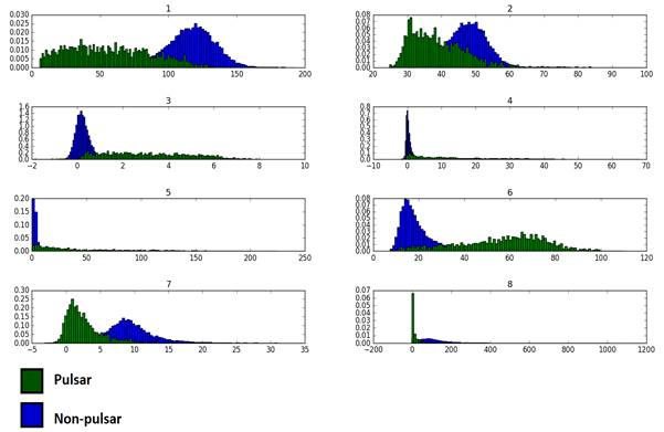
		1	2	3	4	5	6	7	8
Non-pulsars	Kurtosis	0.36	2.35	11.37	59.22	27.19	6.74	2.25	13.62
	Skewness	-0.10	0.43	0.97	4.55	5.04	2.58	0.53	2.77
Pulsars	Kurtosis	-0.81	1.65	-0.88	0.18	-0.06	-0.47	8.60	110.22
	Skewness	0.31	1.04	0.31	0.94	0.96	-0.36	2.27	8.11

For non-pulsars, feature distributions tend to have positive excess kurtosis, in other words they are leptokurtic with tall, distinguishable peaks and long tails. Heavy-tailed distributions such as these tend to have outliers with high probabilities.

For pulsars, on the other hand, peaks are less pointy meaning broader distributions. Platykurtic distributions mostly resemble the uniform distribution. Different pulsars can take an array of different values of similar probability.

Taken together with the largely non-zero skewness values, meaning asymmetric distributions, we can assume that we are dealing with a non-Gaussian distribution which might require some degree of transformation.

The next question that naturally comes to mind is whether there is any separation between the two classes in a statistically significant way. Separation seems a rather nebulous term so it’s a good idea to put some quantitative handles on it. One way to address this is via the Kullback–Leibler divergence which measures how different two distributions are.

High values mean high divergent meaning that it is very unlikely that any values from the tested distribution are derived from the referent distribution. In this case the former are the pulsars and the referent distribution are the non-pulsars. I computed the KL-divergence for each feature.

Significance values were derived by artificially generating a null distribution through 100 synthetic samples (sample size same as number of pulsars in dataset) and then comparing each to the non-pulsar sample. This was repeated for each feature. To get a p-value I calculated the proportion of the generated KL-divergent values which were smaller than the corresponding value for the particular feature. The p-value in this sense represents the occurence of the event given the null distribution.

Based on the aforementioned procedure it was found that all features for pulsars were significantly divergent from non-pulsars. This is good news because it will make things much easier for the classifier to choose a decent boundary for separating the two classes.

It’s also a good idea to visualise our dataset in order to get a decent idea of how the two classes are arranged in the feature space. To do this I used a dimensionality reduction tool known as t-Distributed Stochastic Neighbor Embedding (t-SNE). t-SNE works by trying to find the best fit between a high-dimensional space and a lower-dimensional transformation. First, it models the distribution of inter-point similarities in the original set, p, using a Gaussian kernel and the ones in the projected space, q, with a Student’s t-distribution. The objective now is to find a set of points, y, which minimise the distance between the aforementioned distributions. The cost function is in fact a variant of the Kullback-Leibler divergence which I’ve used here as well. Gradient descent is then employed to find the y–coordinates in the new space. An important hyper-parameter is perplexity (P) which is directly proportional to the variance of inter-point distances. In effect, high values of P will give more weight to global structure while lower values will favour more localised patterns. According to the original authors (van der Maaten & Hinton, 2008) it’s a “measure of the effective number of neighbors” which can determine the spatial arrangement of a particular point and it can typically take values varying from 5 to 50 (although this is not a strict constraint).

Given its relatedness to the methods I’m already taking in exploring the data as well as the fact that it makes no serious assumptions regarding the distribution or the normality of the data, it became a very attractive technique to use.

However, since this is a computationally intense method it was prohibitive to employ it on the entire dataset (for my processing specs at least). For this reason I picked three samples at random, each comprised of 250 pulsars and 250 non-pulsars and used t-SNE on them. Perplexity was set at 30.

We can see that there does seem to be a separation between the two classes. It’s important to bear in mind the particular idiosyncrasies of the visualisation method itself. It would be premature at this point to make any statements regarding the nature of their separation. However, it’s safe to say whatever classifier we use cannot assume a priori that the separating plane is linear.

Feature transformation

Given the nature of the feature distributions, I believe it’s necessary to at least try and transform them into something more resembling of a normal distribution.

I used the following transformation for all features:

Benchmark model

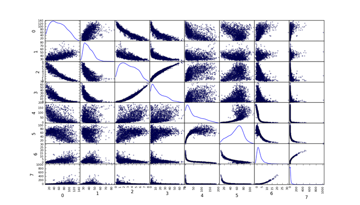
A benchmark model serves to give us a performance threshold. We want the most parsimonious approach at the expense of complexity and processing time. For this reason I chose to use  a multivariable Gaussian classifier. It’s a very intuitive method which affords full transparency into its inner workings. Furthermore it deals well with imbalanced datasets and has been used extensively in anomaly detection problems. A major caveat to bear in mind is that this method assumes that all features follow a Gaussian distribution. This is a bit of a stretch in this case but distributions do not seem to be terribly non-normal. Hopefully the transformations will also help a bit in this regard. The following figures show the correlational matrix between all features for both pulsars and non-pulsars.

Non-pulsars

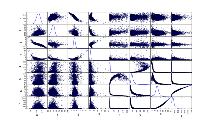
Pulsars

Setting up data

Training took place using k-fold cross-validation. I split up the dataset into 10 folds each comprised of 1620 non-pulsars and 162 pulsars. This was to maintain, roughly, the ratio of the original dataset. One fold was used for testing and the rest of the non-pulsars in the remaining folds were used for training. For each iteration there was a remainder of 59 non-pulsars and 19 pulsars – this was because it was not possible to find a decent number for k with an appropriately sized fold which divided the dataset with no remainder. However taken across iterations, all data points were in the testing set at least once.

Training

The training set consisted only of the remaining non-pulsars. My aim here is to model what a normal, unsurprising data point looks like (cosmic background noise perhaps?) and determine ultimately deviations or anomalies from the norm.

I extracted the parameters of the model, mean for each feature, μ and covariance between all features Σ. Again we’re assuming a multivariate Gaussian but generally the model can deal well (hopefully) with mild deviations. Probability density function is defined as:

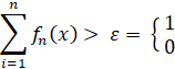
The decision criterion now becomes P(x) < ε. ε is some arbitrary threshold that we can choose empirically. For any value smaller than ε we mark the relative data point as positive – i.e. a pulsar.

Metric

Obviously, accuracy is not sufficient to determine the performance of this method given the skewed ratio of classes. I chose the F1 score which takes into consideration both precision and recall.

The main model: decision trees with bagging

There are two key properties of the dataset we need to take into consideration:

1) imbalance of negative vs positive examples

2) feature distributions are divergent between classes, but they are non-normal.

The standard go-to methods, support vector machines and logistic regression, generally do not deal well with this sort of datasets – especially in the case of imbalanced data. SVMs work well with non-normal data and one could still use a radial basis function to deal with non-linear boundaries in the case of SVMs. Despite this I decided to use decision trees which is a non-parametric method which is gaining a lot of popularity lately and produces much faster prediction latencies.

Granted, the imbalance issue is still pertinent and that’s why I used DTs in conjunction with an ensemble method known as bagging. Bagging is really a meta-algorithm. It’s a way of combining the predictions of a group of weak classifiers into a summative prediction which is generally much more powerful than a single strong classifier.

The above schematic illustrates how bagging is supposed to work. Contrary to another ensemble method, known as boosting, there is no weighting on each of the estimator’s prediction. All predictions for each sample are summed and a classification decision is made based on whether the sum exceeds a specific threshold.

The parameters of the model were number of estimators and the maximum depth of the tree.

Parameter tuning was carried over, 2 to 26 at unit intervals for number of base estimators and 1 to 10 for maximum tree depth (total of 250 parameter combinations).

During the parameter tuning stage, I performed a k-fold cross-validation for each parameter combination. Like the benchmark model, there were 10 folds each consisting of 1620 non-pulsars and 162 pulsars. Training samples were drawn from the remaining 9 folds. Each estimator was trained on a randomly assembled sample from this set (with replacement) consisting of 250 examples from each class. For each parameter combination, I collected the F1 scores and averaged across the testing folds to get an overall performance measure.

The threshold was set at 0.85, meaning that there should be at least 85% of positive “votes” cast from an ensemble of estimators for the example to be classified as a pulsar.

Results: benchmark model

To find the optimum value for ε I ran the model through 250 different values ranging from 10e-8 to 100. Below is a plot illustrating the both the number true positives and total positives at each threshold. Optimum value was found to be at 9.37e-06. However, after some empirical observation it seems that this value is quite volatile from run to run so I rounded it up to 0.001. Generally speaking, anything less than 0.0001 seems to produce very similar results.

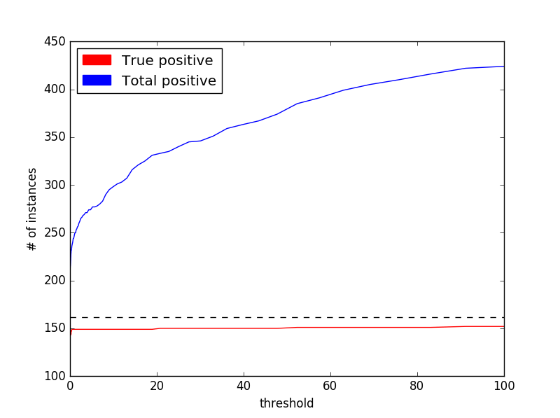
We can see that the main effect is that there is a dramatic increase of false positives with no concurrent improvement in recall. Unsurprisingly the F1 score suffers as well.

As described, the model was tested using k-fold cross-validation with k = 10. Reported performance is the average across all folds for the optimum value of ε.

	At ε = 0.001
F1	0.78
Precision	0.77
Recall	0.8

We can see here that the classifier is doing well at identifying positive cases. Recall score means that it can successfully detect 8 out of 10 pulsars, on average, in a given sample while precision score means that given a positive reading there is 77% chance that it has indeed found a true positive (a real pulsar).

The decent performance scores we are getting here shouldn’t be too much of a surprise since we have already established beforehand that the feature distributions are well separated between class (or significantly KL-divergent). This is not the end of the story however. Although performing at a satisfactory level we still need to make sure that the classifier can pick up on signals which are uncharacteristic of the data we have at our disposal but not classify them as pulsars. After all, it’s a massive universe out there so there’s bound to be more than a few instances which are “anomalous” with respect to our multivariate Gaussian but not real pulsars. How would the classifier perform in such a case?

So it’s important to understand what this specific method is doing in theory. We are essentially attempting to setup a probabilistic model of the universe where there are no pulsars so that anything which deviates from our expected “norm” must be a pulsar. However this is not necessarily true.

To test this I generated 1620 random instances which we know for sure are not pulsars. In fact they could be anything but pulsars. I then added another 162 known pulsars. The question here is: will our model classify the randomly generated instances as pulsars by virtue of their divergent properties compared to the referent distribution?

I tested the model on the dataset and the following is the performance I got:

	At ε = 0.001
F1	0.13
Precision	0.07
Recall	0.78

Performance has fallen quite dramatically. Although, it’s doing a decent job in finding the true pulsars (about 8 in 10), the false positive rate is unacceptably high resulting in a very poor precision score. This means that it’s misclassifying negatives as pulsars when in fact they’re just noisy aberrations from the standard model.

This is a serious limitation of the benchmark classifier and definitely something that has to be addressed in the main model, in addition to improving on the standard performance scores.

Results: decision trees with bagging

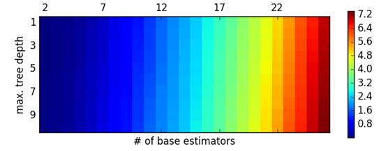
Finding the optimal model involved going through the 15 values for number of base estimators and 7 values for maximum depth yielding a total of 105 different models. The F1 scores are shown below:

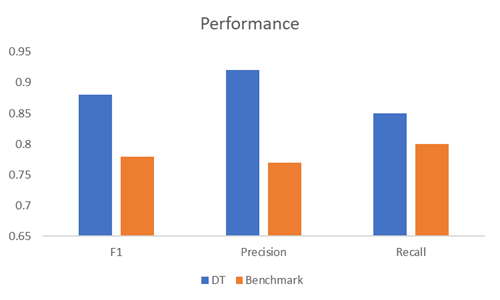
The best model was found to be at 18 base estimators with 7 maximum tree depth (F1 score = 0.881) which exceeds the performance of the benchmark model. I expected a trade-off between the two parameters in terms of variance and bias. Having low tree depth, and thus a “dumber” classifier would give rise to a high-bias model but this could be offset by increasing the number of estimators. Conversely, I did not expect the number of estimators to have a discernible effect on decreasing variance with complex classifiers (high tree depth) so this type of models might be more susceptible to overfitting. By visually inspecting the color matrix above I would say that there seems to be a general peak performance around the reported optimum model (17-18 base estimators at 6-8 maximum tree depth). Generally, simpler models are more affected by poor performance compared to more complex ones.

Finally, there is also prediction latency. Unsurprisingly, the number of base estimators has a strong effect (see below) – as we add more estimators to the model it takes longer to test a sample. For the optimal model, prediction latency for 1782 examples was found to be 0.24 secs (approximately 72161.29 examples / sec). This number is the average across all 10 folds.

Comparatively, the benchmark model was much faster running through the same number of examples at 0.01 secs (approximately 124167.49 examples / sec). Again, the number is the average across all cross-validation folds. As one would expect, the benchmark model is considerably faster given its simplicity. Scaling might become an issue for the DT model, however, if we are dealing with millions of data points.

Finally, I needed to test whether the DT model could deal with data uncharacteristic of the dataset as a whole and correctly classify them as non-pulsars. This is an issue which the benchmark model struggled with so it was paramount to make sure that the DT model could address this successfully.

As in the case for the benchmark model, I generated 1620 random instances and I then added another 162 known pulsars. The DT model did quite well:

There is definitely a massive improvement compared to the benchmark meaning that the DT model can deal well with noisy datasets in extracting true positives.

What about the individual feature contributions? Decision trees assign feature importance values which signify how useful a feature is in regards to classification. In other words, importance quantifies the effect on classification performance after having removed the feature. This is not as same feature relevance which is independent of model bias and refers to the information carried by each feature regarding class.  If we compare these values to the ones calculated earlier for KL-divergence we can see that the single most important feature by far (#3 or excess kurtosis of the integrated profile) is also the second most divergent feature. KL-divergence would be more related to information and relevance described earlier, as well as Gini impurity. The latter is a metric of best separation between classes at different branches of the decision tree.

Conclusions

The aim of this project was to establish a robust machine learning framework to efficiently detect pulsars from a relevant dataset. The model I settled on, decision trees with bagging, managed to attain an acceptable performance. It also showed some robustness when faced with noisy samples which something quite useful considering the source of data we are dealing with.

References

R. J. Lyon, B. W. Stappers, S. Cooper, J. M. Brooke, J. D. Knowles, Fifty Years of Pulsar
Candidate Selection: From simple filters to a new principled real-time classification approach MNRAS, 2016.