Languages: MATLAB, R
Code: https://github.com/A-V-M/past_projects/tree/master/gensem
Summary: A large part of my research as a graduate student in cognitive/computational neuroscience involved thinking a lot about how the human brain represents the rich semantic information which characterises objects in our day-to-day lives. Obviously it’s not all about strict visual processing; there’s something unique going on beyond just seeing an object but understanding what its meaning is within the context of the world we engage with. The following is a shortened report of the conducted work which grappled with these questions during my studies. Specifically, I constructed a computational model, consisting of a 4-layer deep belief network, whose overarching aim is to provide a plausible mechanism under which different levels of semantic representations can arise. I then compared the responses of the model to human behaviour. Finally, I discuss possible practical implementations of the model outside its theoretical implications.

Introduction

Object recognition has made enormous strides in the past few years especially with the advent of deep learning methodologies. However, even though these algorithms are able to successfully identify a visual object, i.e. it has some sort of an internal representation of its visual properties, this does not necessarily imply that it understands the true meaning of what it is seeing. It can’t infer what a hammer is or how it’s used in daily life even if I supplied it with a considerably large number of instances. Computationally instantiable models which can meaningfully organise and recognise objects in the world are crucial if we are to build truly intelligent systems.

Typically object recognition requires the capacities to detect regularities between objects, abstract away from variances in orientations and positions in the visual scene and make reliable inferences against noisy inputs (Kandell et al., 2000). But how do we get a machine to be capable of categorising objects into meaningful compartments of knowledge, such as “animals” and “tools”, which go beyond their mere visual characteristics?

This is actually a complicated problem as it turns out with many possible approaches. Over the course of my PhD I explored a plausible mechanism for this by using Restricted Boltzmann Machines as my cognitive model and then comparing its responses to human behaviour. The hope here is that by gaining some sort of insight into how the brain organises semantic information might help us build truly intelligent machines which can deal with the type of tasks we encounter in our daily lives.

In GOFAI (good old fashioned artificial intelligence) symbolic representations were assumed to be the fundamental substrate of processing. Essentially, processing was interpreted as symbol manipulation demanding a strict set of axiomatic rules in order for concepts to form categories. This is probably not how the brain does it (at least according to mainstream cognitive science; Gardenfors, 2004) which most likely means this is not the most optimal way to go about it either. In deep learning and RBMs it is implicitly assumed that representations are sub-symbolic and feature-based. These can give rise to emergent categorisations via the relatedness between concepts without invoking explicit formalisations.

For my PhD work, features in this case simply meant basic semantic properties such as “has_legs” or “used_for_screwing”. In the case of distributed, feature-based accounts of object representations, similarity between any two objects is typically derived from the overlap of their features (Tversky, 1977; Tversky & Gati, 1978). These feature-based representations give rise to a conceptual space (Gardenfors, 2004) in which the distance between concepts is defined as the degree of feature overlap. This concept of similarity is central to the model’s inner workings. Concepts in this context are assumed to be points within a multi-dimensional geometrical space (Carrol and Wish, 1974, Shepard, 1974).

Data collection

Semantic features were extracted for each object from a set of norms produced by McRae et al. (2005). The authors asked participants to produce a set of features which best characterised a particular concept (e.g. ‘dog’: ‘has fur’, ‘barks’ etc). I used  a British-English version of these norms as formulated in Taylor et al (2012) (concepts unfamiliar to British English speakers, such as “gopher” were removed and concept names were renamed to their British-English equivalent). I used a total of 517 concepts from this corpus for the purposes of the present study. The data was then formalised as a matrix, M, with dimensions c x f, where c signifies the number of concepts (517) and f the total number of features (2341) present across the entire set of concepts. Concepts were represented as vectors of features. Each row in this martix contained the set of semantic features for a particular concept. The row vectors are binary with ‘1’ indicating that a particular feature is true for a concept while ‘0’ denoting the absence of the feature. For example the vector for the concept ‘dog’ would have features such as ‘behaviour_barks’ = 1 and ‘has_a_covering’ = 0.

Sample feature vectors for five randomly drawn concepts. Blue color denotes 0 (or the absence of a feature in the concept) and red denotes 1 (or the presence of a feature).

Deep Belief Networks: Background

DBNs belong to the wider family of generative models (Hinton, 2007). The main aim of this type of model is to learn, in an unsupervised manner, a set of probabilistic transformations which allow the system to infer the probable causes of its input. This places them in distinct contrast to the more standard discriminative models where the aim is to classify input according to a pre-determined set of category labels (Bishop, 2006). Generative models have enjoyed a lot of popularity in recent years, with noted success in the field of computational vision (Kersten et al., 2004; Mumford and Lee, 2003; Dura-Bernal et al., 2012). The main attraction of this type of models is that the algorithms they use introduce a plausible principle of how the brain processes information. Specifically, vision in this regard is understood as a process of inference, whereby the system tries to find simplifying explanations for the incoming, rich sensory data. During this process, the system detects hidden features or patterns within incoming stimuli which allow it to categorise it and identify it accordingly. Perception, in this case, is not seen as a direct mapping between the stimulus and the representation; rather, it is an actively constructive process whereby sensory data guide the dynamic generation of hypotheses by the visual system in order to probabilistically infer what is the most likely stimulus (Rao et al., 2002). In other words, perception is the system’s collective effort to create a coherent picture of its sensory input (Helmholtz, 1878/1971).

This framework has proven especially successful in computational models of low-level vision (Penny, 2010; Hinton, Osindero & Teh, 2006; Ranzato et al., 2007; Bengio et al., 2007). While most studies using generative models have been strictly constrained to vision research, the principles themselves can be applied to any cognitive function (Hinton, 2007). Specifically, the idea that a system can form its own internal representations which contain high-level, and non-linear, inter-correlations between the constituent features of the original input affords itself as a plausible, and testable, account of how the dynamic nature of conceptual representations can arise. I refer to conceptual representations as being dynamic in this context because an intelligent system needs to differentially parcellate information at varying degrees of detail in order to be able to efficiently process and organise the rich sensory input they receive from their environment. To create an effective internal, and coherent, model of the world the semantic system needs to extract multiple layers of representations. These layers are in essence high-level feature detectors whereby higher layers are capable of abstracting away from the original input in such a way that categories can form naturally and without supervision. Ultimately the system learns to categorise input based on the specific featural characteristics of the objects.

Here I will detail the work I have conducted on constructing a generative model of semantic representations. The model itself is based on Geoff Hinton’s work which established the formal basis of deep belief networks. Studies involving DBNs were primarily used to model early visual processes and, to date, have not been applied to conceptual processing.

The work undertaken can be split into three parts and I will go into each one in more detail for the rest of the introduction:

1. Model architecture: where I explain the inner mechanics of the model.
2. Model analysis: where I conduct an analysis of the layers that result from the model and relate the properties of the layers to CSA variables.
3. Model testing: where I compare model performance to previously-collected behavioural (Taylor et al, 2012) data.

Deep Belief Network: Overall architecture

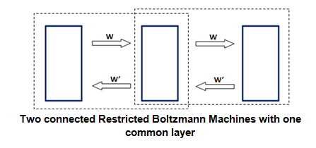
A DBN is essentially a stack of learning modules or layers (Hinton, 2009). Learning in this type of model typically consists of training one pair of layers at a time. A pair of layers is comprised of a “visible” layer (which can be the initial data vector on which the network is trained on) and a “hidden” layer. Both layers are symmetrically connected with a set of weights (i.e. there is a statistical dependency between both sets of units). Each unit in one layer is connected with all the units in the other layer. However there are no connections between units within a layer meaning that their activity is statistically independent. The pair of layers and the general mechanisms of interaction between them are collectively referred to as a restricted Boltzmann machine (or RBM) and it forms the fundamental component of a DBN.

Architecture of the restricted Boltzmann machine. It essentially consists of two layers which are symmetrically connected to each other. The overarching aim is to find an optimal set of weights (W) which allows for the seamless transformation of data vectors from one layer to the other.

Learning with RBMs follows two simple rules: first, all units within the hidden layer of the RBM are updated in parallel following a randomly initialised set of connective weights between itself and the visible layer. The key step following this is that the weights are evaluated on how well they can reconstruct the initial visible layer from the hidden layer. Based on the errors derived from this comparison the weights are updated again and the hidden unit values re-evaluated. The learning is unsupervised because there is no external objective or classification against which the error is derived. This process is repeated until an optimal set of weights is found which can accurately transform the visible layer unit values to hidden unit values and also, even more importantly, the hidden unit values back to the original visible layer. The overarching aim of the RBM is to learn a distribution of possible feature configurations (or states) that the visible layer can take. The basic intuition here is that by going through this learning process, the resulting units on the hidden layer capture high-order, latent features of the initial data structure which would have been otherwise very difficult to uncover (Hinton, 2009; Hinton and Salakhutdinov, 2006).

The learning process within a restricted Boltzmann machine. This cycle is repeated until there is an optimal transformation accuracy between the hidden to the visible layer.

Multiple RBMs can be stacked together. The crucial principle is that each RBM is trained individually with the hidden layer in the first pair becoming the visible layer in the second pair and so on. Once all RBMs have gone through a sufficient number of training cycles (i.e. the weights can transform patterns between layers with near-zero error) the network is now said to be trained. A bottom-up pass within the network consists of using the learned generative weights to get from the initial data vector to the final layer of the network. Conversely a top-down pass consists of using the inverse of the generative weights to re-construct the initial data vector from the top layer of the network. The top-down weights contain a probabilistic model of the training data (Hinton, 2008).

A Deep Belief Net with two passes: one originating from the bottom-layer (far left) towards the top-layer (far right) and one originating from the top-layer towards the bottom-layer. The set of weights connecting pairs of layers learned during the training process are inversed for the top-down pass.

In the model reported here training was based on the entire set of the McRae feature norms which consists of 517 concepts each represented by a 2341-element feature vector. The initial data layer therefore consisted of 2341 nodes. After training, I expected that the top layer of the DBN would capture the intricate semantic relationships between features resulting in cohesive category formations at the expense of fine-grained granularity (i.e. within-category concepts would be highly confusable). This is because the model would be able to uncover statistical regularities across different concepts of a particular category and thus highlight their overall similarities. The McRae dataset, on the other end, represents the finest grained end point of human semantic knowledge since all concepts have a unique combination of features resolving all possible sources of ambiguity.  A top-down pass from the top-layer towards the bottom layer (i.e. the initial McRae feature dataset) would mean that representations become less and less categorically cohesive but gain more distinctive information on individual concepts as the original training dataset is re-constructed.

Model analysis

The model in this case had 4 layers – each of which was built on top of the layer beneath it. As explained in the previous section each layer abstracted further and further from the initial training feature data uncovering high-level inter-correlations between individual features.

Overall architecture of the model.

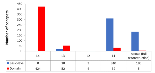
Once the layers had been extracted, their representational structure was examined in detail. Concepts can be categorised at different levels of specificity: superordinate categories such as domain (e.g. ‘living thing’) and general category (e.g. ‘animal’); basic-level (e.g. ‘cat) and subordinate (‘my pet cat’) (Rosch et al, 1976) (note: given the availability of the data at hand subordinate categories cannot be taken into account). How does information content at these different levels of specificity change from layer to layer? I used Shannon’s information theory to determine whether the pattern of response within individual layers contained information about concepts at these three different levels of specificity. In other words at which layer would we have maximal information about an individual concept? Is there a discernible trend of coarse-grained information in L4 towards more fine-grained information in L1?

I also needed to gain an understanding of how concepts were arranged in each layer’s representational space. If we envision the flow of processing within the semantic system as moving from highly categorical types of representation towards more individuated representations then the top-down pass of the model should reflect a similar trend. To address this question I determined the categorical cohesion within each layer’s representational space.

I computed the uncertainty of concept identification at each layer and for two levels of specificity (basic-level & domain). Uncertainty is formally defined as the entropy of the model’s responses (Shannon, 1948; Trappenberg, 2009) and is essentially an indication of the model’s confidence in making a response. For example, in situations where the model is faced with a multitude of equally-likely candidates would lead to high uncertainty. I reasoned that as the flow of processing progresses along the top-down pass of the model, uncertainty regarding the precise identification of a concept would decrease for each individual layer. For example in uniquely identifying a ‘tiger’ from a ‘lion’ the semantic system requires full access to the semantic features which constitute the ‘tiger’ concept. This is because there are many features in common between the two concepts. To resolve uncertainty in this case the semantic system would need to resort to those neural structures which carry sufficient information to make the distinction. Increased fine-grained information on individual concepts means decreased uncertainty regarding precise identification at a specific level of specificity. Uncertainty, in combination with identification accuracy, formed the quantitative indices of the model’s performance. High performance in this case equates to highly accurate responses with low uncertainty.

Methods

I constructed a deep belief net consisting of four layers. The number of units within each layer is arbitrary although generally it is advised that it is smaller than the number of features in the training data set (Bengio, 2007). The expectation during the training process is that by forcing the initial data into a vector with fewer elements, hidden features of the data can be revealed. It is useful to imagine this process as a non-linear version of principle components analysis (PCA; Hinton and Salakhudinov, 2006; Bengio, 2007) where the principal components embody the main sources of variation within the data. In this sense, each layer unit captures a specific principal component of the data.

The network was trained on the full McRae feature norm dataset (517 object x 2341 features). The 517 objects were also split into 24 categories as well as into 2 domains (i.e. living / nonliving). This was done to test the model at different levels of specificity – basic-level (n = 517), category-level (n = 24), and domain-level (n = 2). Objects were grouped in categories and domains by hand. All code was written in MATLAB (v8.3) and parts of it were based on Hinton and Salakhudinov (2006).

First, I will describe how the model was trained along with the basic rules of learning that were used. I will then describe how I analysed the representational content within each of the resulting layers in order to: 1) determine the level of specificity appropriate to each layer using Shannon information, 2) investigate the performance of individual concepts with uncertainty measures. I finally compare these extracted measures against behavioural data.

Layer formation and analysis

Deep belief nets are trained in a sequential fashion where each trained layer is used as input for the layer above it. Each pair of layers forms an RBM and training is carried out one pair at a time. Each newly trained layer is then ‘stacked’ on top of the preceding one which is then subsequently used as the training set for another layer above it. At the end of the process the initial training data is transformed during a bottom-up pass, from layer to layer, by a set of trained weights.  A top-down pass from the top-most layer will, conversely, re-construct the initial data set (i.e. the McRae norm dataset).

The model comprised of four layers (plus the initial training dataset) numbered L4 (as the top and final layer) to L1 (the first layer formed during training and the only layer in direct interface with the initial dataset). The reason there were only four layers was two-fold: first, there is an upper limit on the number of layers imposed by the nature of the dataset itself. Typically, models such as these are trained on a vast number of stimuli with a relatively small number of features (Bishop, 2006; Hinton, 2007). For example, the image training set used in Hinton and Salakhutdinov (2006) comprised of 20,000 images each made out of 784 pixels. The model itself comprised of one data layer and three hidden layers which was sufficient for the study’s purposes. By contrast, the present dataset comprised only of 517 concept-vectors each with 2341-elements. In this case, having more than four layers would have resulted in poorer reconstruction accuracy. This is because the connecting weights between further layers would not be sufficiently trained given the nature of the training data. Secondly, given that this model is in an early stage of development, it is better to have fewer layers which are more manageable during analysis compared to a vast number which would have made a thorough analysis intractable. For the present study the flow of conceptual processing in the ventral stream was modelled as the flow of information from L4 to L1 (i.e. the top-down pass). This means that both during testing and analysis the aim was to go from a highly abstract, categorical representation (in the top-most layer or L4) towards representations which resemble the highly differentiated, fine-grained nature of the initial training data.

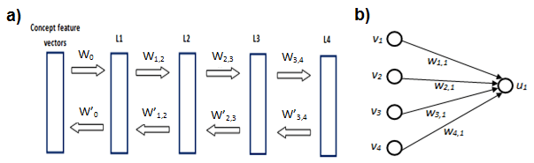
a) Overall architecture of the model which consists of one input layer (with 2341 features) and 4 ‘hidden’ feature layers (each consisting of 750 units). In the present study the flow of processing is simulated as going from L4 towards L1. b) A simple 4-unit layer which is fully connected to a unit () belonging to the layer above it. None of the units () within the layer are connected to each other but they are all connected to the unit above making the probability of its activation statistically dependent.

I ran the model on three different unit numbers [500, 750, 1250] where 750 was the setting with the smallest amount of reconstruction error. The number of units was kept constant for all layers. I did this to remove any implicit assumptions regarding the neural size of the processing regions along the ventral stream.

There was no dependency between units within layers, because there were no connections between units within a layer. A unit can take a value of either ‘0’ and ‘1’ with a certain probability, . However, as the equations below show, the activity of units across two adjacent layers is dependent. In other words the conditional probability, , is directly computable if we know the states of the layer units beneath. However we cannot compute such a probability for units belonging to the same layer. This is because there are no connections between neighbouring units within a layer but any given unit receives a collective input from all the units belonging to the layer beneath it. The weights were learned between layers over 250 epochs, with the weights at the 250^th epoch being used as the final set of weights. The number of training epochs was derived during initial trial runs. Further epochs did not substantially improve in reconstruction errors. The probability with which a certain unit was activated was computed by:

(Eqn. 1)

The σ function in this case signifies the logistic function:

(Eqn. 2)

This function confers a non-linear stochasticity on the overall activity pattern for each layer. b_j is the bias for unit u_j and w_ij is the weight between units v_i and u_j. The result of these equations is that unit activity is: a) stochastic and b) defined by the linearly weighted sum of all the unit states of the layer beneath it.

The training for the connective weights between layers was derived from the following formal learning rule:

(Eqn. 3)

For every training cycle within a single RBM there is one bottom-up pass for every top-down pass.  is the correlation between the two units during training from initial data. The objective in this case is to find a weight value which ensures that this correlation is maintained when doing a reverse, top-down pass. When the result of the subtraction operation is zero or near-zero then the weight values have reached their target. All the information necessary to transform representations from one layer to the next is contained within these weights. Even there is a loss of information or ‘corruption’ during training it can be recovered because of the weight-matrix transformations.  is the learning rate which for the present modelling study was an exponential function with the initial value set to 1. This was done to give decreased importance to later stages of the learning process and avoid over-training.

Information theory

A concept is represented as a particular pattern of activation within each layer.

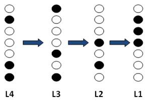
These patterns contain information about a particular concept. I needed a way to quantify this information and assess it for different levels of specificity (basic-level, category, domain). The goal was to investigate whether there was a meaningful trend of information flow from L4 (top-most layer) to L1. Specifically I asked: how much information could I extract about a concept at a given level of specificity (e.g. which level can answer the question,  ‘is it a living thing?’ / ‘is it an animal?’ / ‘is it a dog?’) just by observing its associated activity pattern on a particular layer? This question is formally defined as the mutual information between concept C_i and the model layer response R_i. Mutual information, I(C; R), is defined as (Mackay, 2003):

(Eqn. 4)

H(S) is Shannon entropy (or maximum entropy; Cover and Thomas, 1991) which is the entropy when each category is equally likely and is the average amount of information contained within a particular dataset. This value is directly related to the number of possible choices – high numbers give rise to higher entropy values since there is a larger margin for error.

(Eqn. 5)

Given this equation, if the model is faced with a particular response pattern and asked to make a guess regarding the precise basic-level identification of the concept there would be a total of 517 possible candidates (i.e. the total number of unique concepts within the McRae norms set all with the same probability) giving rise to high stimulus entropy. On the contrary, domain-level decisions (living vs. nonliving) are effectively binary and as such have relatively low entropy. Fewer choices means that one is much less likely to make an error. The higher the value in n (the number of possible distinctions; see Equation 5), the higher the stimulus entropy.

The second term in Equation 4 is the conditional entropy. It quantifies how much information remains unaccounted, regarding the identity of concept C after observing response R. It is generally defined as:

(Eqn. 6)

P(u) is the overall un-conditional probability of getting a particular pattern of response across the entire set of units of a layer, i.e. . This equation provides the value for  after the model is fully trained. P(Cn|u) is the conditional probability of observing a particular concept given the specific response. How this probability was computed is described in the following section.

Bayesian inference

In making a decision regarding a concept’s identity the model needs to infer a probability distribution across the entire set of possible candidate concepts. This means that the model has to compute the conditional probability of a concept given the specific activity pattern elicited across a layer. The winning candidate is the concept with the highest conditional probability.

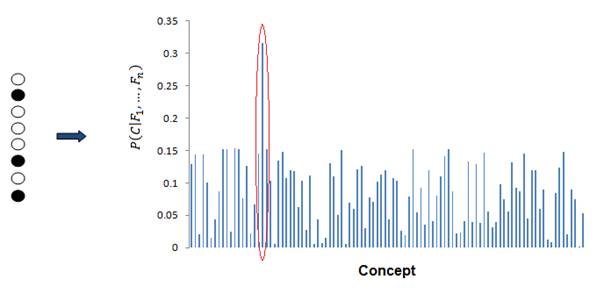
A simplified example of how the model makes a decision given a particular activity pattern. It will compute a conditional probability over the entire set of concept and then pick the winning candidate scoring the highest (circled in red).

The conditional probability can be generally defined as:

(Eqn. 7)

P(C) in the above equation is the unconditional probability of getting a particular C concept which is computed as 1 / n (n = number of concepts = 517).  Although this is the standard equation for Bayesian estimation of a conditional probability it was preferable to use the following equation mainly because there were a smaller number of terms involved:

(Eqn. 8)

P(Fj|C) is the likelihood of observing an activated unit, Fj, if presented with concept C.  This probability is already known through Equation 1 which explicitly computes the activation function of an individual unit during training. Each concept vector within a layer comprises of a set of probabilistic values. I used these values to extract P(Fj|C). P(Fj|~C), in this case, is simply: 1 – P(Fj|C).

Both are instantiations of a naive Bayes classifier. This type of classifier is specifically referred to as ‘naive’ because of the strong assumption that the units within a layer are independent (Bishop, 2006) which is actually the case in this model. This method was crucial in determining the accuracy of concept identification within each layer of the model because the winning candidate was defined as the concept with the highest posterior probability. During each test run each concept was run through each layer of the model. The winning candidate was then recorded to assess the layer’s performance. Accuracy was then defined as the number of times the model’s winning candidate was the correct concept divided by the total number of runs.

The method so far only extracts a probability distribution over basic-level categorisations (e.g. ‘dog’, ‘peacock’ etc). The model also needs to decide at domain (‘living’,’ nonliving’). In order to do this I converted the computed conditional probability for a basic-level identification, P(C|F1,…,Fj), into a conditional probability for a domain-level identification. In other words given a particular activity pattern, {F1,…,Fj}, what is the most likely domain to which a particular concept might belong to?

P(CAT|F1,..,Fj) was defined by the following matrix operation:

(Eqn. 9)

P is an -element vector containing all the probabilities across the entire concept set. M is a  matrix containing all category membership information across the entire concept set (the membership matrix).  in this case is the number of categories and the number of conceptsThe membership matrix was normalised across each (category) column by the total number of concepts within each category. This was done to make sure that all probability vectors for each category had a total sum of 1. This function is effectively a summing operation: if the model produces a large number of high-probability candidates within a particular category then they will collectively give rise to a high probability for that category being the winning candidate. There was one non-standard category containing 92 objects (‘miscellanea’) which were not easily put into a recognisable category. This was removed from any further analysis. For domain, the membership matrix was a 2 x 425 binary matrix; 2 being the number of domains (living and nonliving).

Uncertainty and confidence measures

Uncertainty is closely related to information as defined in Equation 4 as well as the naive Bayes classifier described earlier. Using the probability vector, P(Cn|F1,..,Fj), as a starting point we can derive a measure of uncertainty as:

(Eqn. 10)

H(Cn) measures the degree of entropy across the concept probability vector. High entropy means that the pattern activity derived from the model layer contains little information. Low entropy means that there are only a few competing high-probability candidates. Zero entropy means that the probability distribution has collapsed to just one winning candidate at a probability of 1 with all other candidates having a probability of 0. The maximum value for H(Cn) is equal to the stimulus entropy H(S) defined in Equation 5. Entropy, as calculated and defined in this section, is what I refer to as uncertainty throughout this chapter.

Uncertainty is measured in bits which might be difficult to interpret intuitively. For this reason I also computed a further measure where values ranged from 0 to 1. I simply divided a concept’s uncertainty score by the stimulus entropy (see Eqn. 5):

(Eqn. 11)

Confidence, N(Cn), in this sense denotes the degree of variance within the entire concept set that is accounted for by the response pattern within a layer – when there is little variance, confidence will be high and vice versa. In combination with accuracy, confidence provides a quantifiable measure of the model’s overall performance – high performance means high accuracy with high confidence / low uncertainty.

I first ran a top-down pass to determine reconstruction accuracy at L1 with a 80-20 cross-validation split. This was found to be 91%. This level of accuracy means that the model was able to recover information closest to the original training data set. Most importantly, this is a strong indication that the weights have been trained adequately and the layers are suitable for further analysis.

There were four analyses in total conducted on the model to assess: a) information content b) overall performance (i.e. accuracy and uncertainty) c) representational structure and d) the relationship between feature statistics and performance. The following sections are devoted to presenting the results from the layer-by-layer analysis.

Information content

I used mutual information between layer responses and concept identities to assess the information content at each layer and for all three levels of specificity.

Line plot showing the trend of information content from L4 to L1.

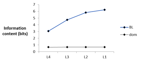
The averages across layers for different levels of specificity were: 4.96 bits for basic-level, 3.04 bits for general category and 0.67 bits for domain. This difference in bits across levels of specificity was due to differences in stimulus entropy. Unsurprisingly, the large number of possible choices for basic-level (n = 425) meant that it had the highest stimulus, or theoretical maximum, entropy with domain-level the lowest. I decided to normalise each specificity level by the stimulus entropy. A score of 1 in this case would be the ceiling of how much information content is possible to represent. The figure below shows that all layers are near-ceiling for domain-level identifications (mean: domain = 0.97) but only L1 reaches a comparably high degree of information for basic-level (0.99).  Overall, information content for levels of specificity increases from L4 to L1 but this trend is much more pronounced for basic-level.

Line plot showing the trend of information content normalised by stimulus entropy from L4 to L1.

Accuracy

Accuracy was defined as the proportion of correct predictions made by a particular layer while uncertainty is a characterisation of the probability distribution. I collapsed the performance measures across all 25 runs and 517 concepts into a grand mean for each layer and specificity level. This resulted in a total of 12 values (4 layers x 3 levels of specificity) for each measure. L4 was the worst performing layer overall with accuracy reaching chance-levels (54.5%) for basic-level and moderate levels (70.5%) for general category. Domain-level performance remained near ceiling across the entire top-down pass (mean: 98%) while basic-level performance was lower (88% and 81% respectively).

 (top) Bar plot indicating the average accuracy scores for all layers at three different levels of specificity. L4 is the first stage of the top-down pass carrying the most general, coarse representations while L1 is the layer most closely related to the initial concept dataset. (bottom) Bar plots for domain and L1 accuracy at different axis ranges in order to highlight the fine difference across layers for the former and across specificity levels for the latter. Standard error bars were not included because of their extremely small size (<<0.01).

Types of error for basic-level identification

There were three types of error the model could make when identifying concepts at the basic-level – within-category, within-domain and across-domain. L4 made the highest, overall, number of errors with L1 the lowest.

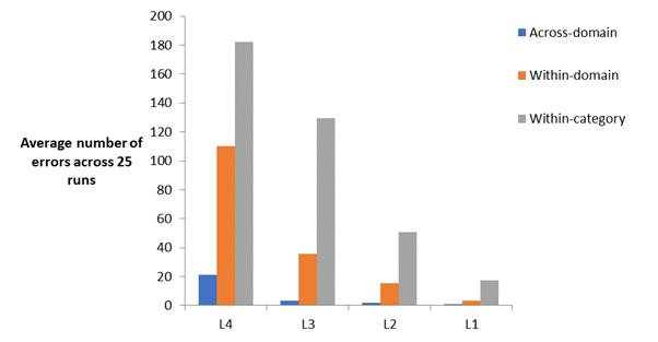
Average number of the three types of errors across 25 runs for all four model layers.

Most importantly, L4 had the highest proportion of within-domain errors (35%) vs. L1 which had the lowest (16%). On the other hand, L1 had the highest proportion of within-category errors (80%) vs. L4 which had the lowest (58%). This means that the specificity of the responses became increasingly more refined: if the model made an error at L4 it was likely to be broadly within the correct domain but not necessarily within the correct category. Conversely at the end-point of processing, at layer L1, errors are more likely to be within the correct category. Proportion for within-domain/within-category errors for layers L3 and L2 was comparatively the same with 21%/77% and 23%/75% respectively.

Effect of layer on overall accuracy

I computed the overall, average accuracy (across all specificity levels) within each layer: L4, 73.5%; L3, 88.4%; L2, 95.8%; L1, 98.6%. I then ran a Kruskal-Willis test (nonparametric one-way ANOVA which does not assume a normal distribution) to determine whether there was an overall effect of layer on the average accuracy (χ² (1550) = 1351.77; p << 0.01).

Effect of layer on accuracy within individual specificity levels

I ran three Kruskal-Willis tests, one for each specificity level, to determine the effect of layer on the accuracy of individual specificity levels. I found that layer had an effect on accuracy for all specificity levels (basic-level: χ²(2067) = 1271.6, p << 0.01; domain: χ² = 408.43, p << 0.01). For domain, although the effects are significant the actual effect size is small. This is probably due to the extremely small standard error values for each layer (L4 = 0.0024; L3 = 0.0015; L2 = 0.0012; L1 = 0.0008).

Effect of specificity level on accuracy within individual layers

I ran four Kruskal-Willis tests, one for each layer, to determine the effect of specificity level on accuracy within individual layers. I found that specificity level had an effect on accuracy within all layers (L4: χ²(1550) = 766.34, p << 0.01; L3: χ² = 706.46, p << 0.01; L2: χ² = 332.3, p << 0.01; L1: χ² = 99.21, p << 0.01). L1 performs very highly for all levels of specificity – as with domain the actual effect size is small but still yields a significant effect across levels due to small standard errors (basic-level = 0.0013; domain = 0.0008).

Uncertainty

Bar plot indicating the average uncertainty scores for all layers at three different levels of specificity.

Uncertainty is closely related to information so it was expected that the average score for each layer would follow the trends for information content for both levels of specificity. Again the most pronounced change across layers was exhibited for uncertainty at the basic-level reaching its lowest point at L1 (0.55 bits).

Effect of layer on overall uncertainty

Again, as with accuracy, I averaged all uncertainty values within layers. A Kruskal-Willis test revealed a strongly significant overall effect of layer on average uncertainty (χ² (1550) = 3410.95;  p << 0.01).

Effect of layer on uncertainty within individual specificity levels

Similarly when the same test was run within individual levels of specificity there was a strong effect of layer on uncertainty (basic-level: χ² (2067) = 1220.62; p << 0.01; p << 0.01, domain: χ² = 1141.7; p << 0.01).

Effect of specificity level on uncertainty within individual layers

I ran four Kruskal-Willis tests, one for each layer, to determine the effect of specificity level on accuracy within individual layers. I found that specificity level had an effect on accuracy within all layers (L4: χ² (1550) = 1335.29, p << 0.01; L3: χ² = 1171.64, p << 0.01; L2: χ² = 1098.91, p << 0.01; L1: χ² = 938.64, p << 0.01).

Summary

Taken collectively both performance measures indicate a clear pattern of performance from L4 to L1. L4 overall had the greatest differentiation in performance across levels of specificity on both uncertainty and accuracy. L1 provided highly confident and accurate responses across the entire hierarchy of conceptual specificity. This is not surprising if the results for information content are taken into account since they clearly indicate an increasing trend of information for all levels of specificity which is especially pronounced for basic-level.

Category cohesion

Category cohesion was measured by the Davies-Bouldin index – the lower the index the higher the cohesiveness. I also included the initial McRae feature vectors in the result for comparison. There was a trend of decreasing cohesion from L4 to L1.

Category cohesion measures for all model layers and initial training dataset.

Testing the model against behaviour

The original behavioural study by Taylor et al was conducted to find out whether feature-statistics have an effect on how conceptual representations are processed in the brain under different task-demands. It comprised of two experiments: a basic-level naming task and a domain decision task. For the first experiment participants had to verbally identify a set of 412 images at the basic-level of specificity, while for the second a different group of participants had to press a button which denoted whether the depicted concept was a living or nonliving thing.

In this study, I tested whether the time taken for a participant to make an identification (either at basic or domain) was related to model performance.  Processing at each layer in the model involves the prediction of the most likely concept given a particular response. The confidence of the model in its prediction at each layer would determine the extent of processing that needs to be undertaken. High uncertainty would necessitate further processing until a sufficiently refined probability distribution yields a confident prediction. In this case, I reasoned that the time taken to produce a response (behavioural RTs) in humans would be directly related to concept uncertainty derived from the model. This is because the overarching purpose of both the model and the brain’s object processing system is to resolve uncertainty: a concept with high uncertainty will require further processing – or more time in the participant’s case – to disambiguate it from semantic neighbours and thus maximally increase confidence in its prediction. To test this claim I compared human reaction times against two performance measures from the model: earliest layer response (ELR) and uncertainty. My expectation was that if a particular aspect of human behaviour can be reproduced through the model’s responses then it would strongly suggest that uncertainty, and its resolution over the course of processing, play a decisive role in object recognition.

ELR was defined as the earliest layer (with L4 being the absolute earliest and L1 the latest) at which the model made a correct response (for basic-level and domain-level) at >90% confidence. Confidence was defined as uncertainty normalised by stimulus entropy at a particular level of specificity. ELRs were used as a proxy for the model’s “reaction time”. The model had four layers each effectively a stage of processing. Low ELRs mean that the model is able to make highly confident, correct responses with information available within the initial stages of the top-down pass (i.e. either L4 or L3). High ELRs mean that the model requires more fine-grained information only available within the latter layers, or even a full reconstruction of the McRae feature norm vector. I then tried to determine whether the model ELRs were able to capture a signification portion of the variance within the actual reaction times of human participants. When identifying objects at the domain level the model would only recruit information at the earliest layers along its top-down pass. Conversely, when identifying objects at the basic-level the model would recruit information at further layers towards L1. Overall, concept-specific ELRs should correlate with concept-specific RTs.

Uncertainty is a measure of central importance within the computational mechanisms of the model. It was shown that uncertainty across all levels of specificity decreases from L4 to L1. If a concept is cohesively embedded into its category by means of a high number of shared features it will generally have a comparatively high (basic-level) uncertainty. At layers L2 and L1, as information becomes more refined and detailed, a concept becomes detached from its category and only the most similar concepts remain within its immediate neighbourhood. Uncertainty in this case is driven by only the closest, immediate semantic neighbours of a concept.

I argued that these different types of layer-specific uncertainty would have a differential effect on reaction times. In other words, reaction times in this case are effectively a reflection of the types of uncertainty that need to be resolved. When participants are making a domain-level decision their reaction times would largely correlate with domain uncertainty at L4. At this layer, information is coarse-grained but highly ordered categorically. Domain-level uncertainty at L4 signifies how well the system can ascertain whether a concept is living or nonliving. The extent of processing will depend on the degree of uncertainty at this early stage. Low uncertainty will result in short reaction times while high uncertainty will necessitate further processing and so longer reaction times. However uncertainty at L1, which signifies the end-point of processing within the model, will have no relationship to behavioural performance for domain decisions. This is because L1-uncertainty, as mentioned earlier, is highly dependent on the closest, immediate semantic neighbours of a concept. It is not necessary for the system to disambiguate a concept at this level of granularity.

I also tested whether there was any relationship between basic-level naming reaction times and the model’s uncertainty when making basic-level identifications. Within the context of the model, basic-level naming necessitates resolving uncertainty at a very fine-grained level of specificity. I reasoned that to make a basic-level distinction the semantic system must be able to disambiguate a concept from other competitors which are very similar to it semantically – considerably more similar compared to other members of its category. This means that uncertainty at this level will not be captured in L4, which only has the capacity for general, abstract representations, but rather in L1 – the end-point of processing in the model. I argued it would take more time for participants to process and identify an object with high L1-uncertanity as derived from the model. L4-uncertainty, in this respect, has no relevance since L4 is at a stage of processing which has a limited representational capacity. The demands of the task are such that necessitate further processing beyond the stage encapsulated by L4.

In summation, I carried out two different tests against behavioural data:

1. Extraction of ELRs at two different levels of specificity (basic-level and domain) and comparison against the corresponding behavioural reaction times.
2. Correlation between uncertainty at domain-level (for layers L4 and L1) and the corresponding reaction times in the second task of the study. Similarly, a correlation between uncertainty at basic-level (for layers L4 and L1) and the corresponding reaction times in the first task of the study.

Behavioural data collection

Inverse-transformed reaction times were collected from each participant from both tasks performed during the Taylor et al. study. There were a total of 412 stimuli for basic-level and 475 stimuli for domain-level. For basic-level, stimuli which had below 70% identification accuracy across all participants were automatically removed from the entire dataset before any further analysis.  Stimuli consisted of coloured pictures, centred against a white background. All stimuli were derived from concepts found in the McRae norm database (see Taylor et al., 2012 for full details).

Participant responses were analysed separately. For each participant, stimuli with incorrect responses, stuttering (for basic-level task), or reaction times faster than 300msec or longer than 4s were removed and analysis was performed on the remaining data (average number of stimuli across participants: Basic-level = 220.5 / Domain = 410.5).

Extracting Earliest Layer Responses (ELRs)

I ran the full model a total of 25 times for both basic-level and domain-level identifications. It was noted that concepts belonging to the ‘miscellanea’ category which contained un-categorised objects were removed from the analysis. However, I had to include the category in the present study because a high number of these concepts were included in the domain-level task in Taylor et al (2012). Including this category meant that the total number of concepts during the model run totalled to 517 (vs. 425 in the previous chapter). For each concept, the run was stopped if a layer fulfilled the following two conditions: 1) correct identification and 2) confidence level above 90%. The number of the layer, at which these conditions were satisfied, was then recorded. The chosen confidence threshold means that there is a 90% reduction in the overall uncertainty of the model layer given the response elicited by the concept. Lower thresholds, tending towards 0%, would mean that if a layer produces a correct response it becomes increasingly likely that it was made at random. Responses at lower confidence thresholds would be highly inconsistent in this respect. I chose a confidence threshold of 90% to ensure that responses would be consistent across runs. Layer numbers were recorded according to their order in the sequence of processing (L4 = 1; L3 = 2; L2 = 3; L1 = 4; full re-construction = 5). The ELR for a particular concept was then computed as the median layer number across runs. There were two sets of ELRs (each comprising of 517 concepts), one for basic-level and one for domain-level. I then extracted the values for concepts which were found in either task.

Uncertainty measures

I derived a value for each concept at layers L4 and L1 for each corresponding specificity level. This resulted in a total of four variable sets (2 x 412 uncertainty values for the basic-level task; 2 x 475 for the domain-level task).

Mixed effects model

To assess the relationship between model-derived measures and behavioural reaction times I performed a linear mixed effects model across all participants using the same procedure as in the Taylor et al study within the R programming environment (R Development Core Team, 2008). Behavioural responses (inverse-transformed reaction times) were the dependent variable for all subjects. Independent variables, for each subject, comprised of either ELRs or uncertainty (i.e. the variable of interest) plus a further 8 control variables which were computed and used in the original study, namely phonological length, visual complexity, naming agreement, lemma frequency, familiarity, cohort size and H-statistic. This was done to remove any visual, phonological or lexical effects from the responses. Mixed effects models incorporate both fixed (i.e. individual variables) and random effects (i.e. subjects) within the same statistical framework. The method takes into account individual fluctuations across the entire group as well as variation in the overall mean of individual predictors (Baayen, 2008).

The analysis was split in two parts. First, I investigated whether the speed at which participants made a response, for either basic-level or domain, was related to the earliest layer at which a model made an accurate and confident response. For the second analysis, I assessed the relationship between uncertainty, derived from two different layers (L4 and L1), and the reaction times. For both analyses, I made use of a linear mixed effects model.

Earliest Layer Responses (ELRs)

I extracted ELRs for both basic-level and domain-level for all 517 concepts in the McRae feature norm dataset. First, I plotted the distribution of responses for each specificity level. I then used a χ²-test of independence to determine whether there were any significant differences between the two response distributions. I found that there was indeed a strongly significant difference (χ²(4) = 838.16; p < 0.01): overall the model was “faster” in performing domain-level identifications since it was able to make accurate and highly-confident responses at L4. Only 1% of concepts required a full reconstruction of the McRae feature vectors meaning for the vast majority of concepts (82%) the information contained in L4 was sufficient to make a domain decision. For basic-level, 96% of concepts required the fine-grained information contained at the very latest stages of processing with 36% reaching full reconstruction.

Histogram of ELR distributions for both basic-level and domain.

Model ELRs vs. behaviour

There were two sets of ELRs – one for each specificity level – extracted over the whole 517-concept dataset. Given the skewed distribution of the ELRs I decided to transform by squaring each value to make the data more suitable for statistical analysis. The results summarised in Table 1 are based on the transformed ELRs.

	Basic-level				Domain-level
	Estimate	Std. Error	t-value	p-value	Estimate	Std. Error	t-value	p-value
(Squared) ELRs	-0.004	0.001	-2.977	0.003	-0.011	0.002	-5.114	0.000
Additional control variables
Phonology	0.004	0.007	0.593	0.553	-0.006	0.009	-0.699	0.485
Visual complexity	0.000	0.006	0.020	0.984	0.024	0.009	2.749	0.006
Naming agreement	0.115	0.020	5.595	0.000	-0.030	0.009	-3.371	0.001
Frequency	0.049	0.007	7.353	0.000	-0.029	0.009	-3.225	0.001
Familiarity	0.079	0.007	11.832	0.000	0.025	0.009	2.762	0.006
Cohort size	-0.017	0.007	-2.551	0.011	-0.019	0.009	-2.103	0.036
H-stat	-0.019	0.008	-2.340	0.020	-0.025	0.009	-2.774	0.006
NOF	0.028	0.007	4.192	0.000	0.033	0.009	3.729	0.000

Table 1: Results from the mixed effects model showing coefficients for all control variables and ELRs. P-values were estimated in the R programming platform using the Satterthwaite approximation (Satterthwaite, 1946).

Squared-ELRs for both basic-level and domain were found to be significantly correlated with behavioural reaction times (t = -2.98** / t = -5.11** respectively). The direction of the effect in both cases is negative because the dependent variables in all cases are the inverse-transformed reaction times (had it been the raw reaction times there would be a positive correlation). In follow-up analyses, the raw ELRs were also found to have a significant effect, t = -2.6** and –4.9**, for basic-level and domain respectively. Overall, these results show that concepts which engage later layers in the model also correspond to longer RTs for participants.

Mixed effects model: Uncertainty vs. behaviour

	Basic-level				Domain-level
	Estimate	Std. Error	t-value	p-value	Estimate	Std. Error	t-value	p-value
uncertainty.L4	0.0221	0.0160	1.3810	0.1684	-0.0637	0.0113	-5.6360	0.0000
uncertainty.L1	-0.0611	0.0176	-3.4770	0.0006	-0.0034	0.0114	-0.2960	0.7677
Additional control variables
Phonology	0.0021	0.0065	0.3180	0.7507	-0.0049	0.0087	-0.5670	0.5709
Visual complexity	0.0008	0.0063	0.1270	0.8987	0.0234	0.0086	2.7300	0.0066
Naming agreement	0.1075	0.0205	5.2520	0.0000	-0.0288	0.0087	-3.3060	0.0010
Frequency	0.0458	0.0067	6.7880	0.0000	-0.0282	0.0087	-3.2320	0.0013
Familiarity	0.0790	0.0067	11.8650	0.0000	0.0277	0.0089	3.1230	0.0019
Cohort size	-0.0182	0.0067	-2.7350	0.0066	-0.0183	0.0087	-2.0960	0.0368
H-stat	-0.0223	0.0081	-2.7360	0.0065	-0.0252	0.0087	-2.8890	0.0041
NOF	0.0271	0.0066	4.0810	0.0001	0.0320	0.0087	3.6720	0.0003

Results from the mixed effects model showing coefficients for all control variables and both uncertainty values for the respective layers. P-values were estimated in the R programming platform using the Satterthwaite approximation (Satterthwaite, 1946). Values highlighted in red indicate the type of uncertainty which was predicted to have an effect at that particular specificity level.

L1-uncertainty had a significant effect on basic-level responses, where greater uncertainty was associated with longer RTs (t = -3.48**) but no effect on domain-level responses (t = 1.38). In the same fashion, L4-uncertainty had a significant effect on domain-level responses (t = -5.64**) but no effect on basic-level responses (t = -0.3). Most importantly, the type of uncertainty was selectively correlated with the type of task taking place: L1-uncertainty with basic-level and L4-uncertainty with domain. As with ELRs the direction is negative, meaning that there is a positive dependence between the actual non-transformed reaction time and uncertainty. These results show that both types of uncertainty can reliably predict the time taken for participants to respond.

Concluding remarks

The aim of the study was to show that an aspect of human behaviour (reaction times) during object recognition can be adequately modelled and predicted computationally. Each layer of the 4-layer deep belief network exhibited distinct representational profiles. At L4 representations were more “economical” yet sacrificing detail. As representations flowed from L4 to L1 there was an observed trend of decreased uncertainty and increased accuracy for specific identification of objections. Domain identification was not affected. I see this study as an example of trying to predict human behaviour not by using a descriptive model but instead an explanatory, generative model which can theoretically mimic how human brains actually work. We have seen that both ELRs and layer uncertainty are strongly correlated with reaction times. However, although this is suggestive of the model’s predictive capacities, we would still have to apply some of cross-validation before making any strong claims.

In summation, these results suggest that RBMs can privide a solid, computational framework for modelling semantic representations. Practical applications are varied but models such as this one could be applied in situations where the objective of the processing system is to resolve uncertainty.

References

Björck, Å. (1996). Numerical methods for least squares problems. Philadelphia: SIAM.

Davies, D. L., & Bouldin, D. W. (1979). A cluster separation measure. IEEE Transactions on Pattern Analysis and Machine Intelligence , 2, 224-227.

Donderi, D. (2006). Visual Complexity: A review. Psychological Bulletin , 132, 73–97.

Friston, K., Henson, R., Phillips, C., & Mattout, J. (2006). Bayesian estimation of evoked and induced responses. Human brain mapping , 27 (9), 722-735.

Gärdenfors, P. (2004). Conceptual spaces: The geometry of thought. MIT press.

Harnad, S. (1990). The symbol grounding problem. Physica D: Nonlinear Phenomena , 42 (1), 335-346.

Harrell, F. E. (2013). Regression modeling strategies: with applications to linear models, logistic regression, and survival analysis. Springer Science & Business Media.

Helmholtz, H. (1878). Selected writings of Hermann von Helmholtz (1971). In The facts of perception (pp. 366-408).

Hinton, G. (2009). Deep belief networks. Scholarpedia , 4 (5).

Hinton, G. E. (1986). Learning distributed representations of concepts. Proceedings of the eighth annual conference of the cognitive science society , 1 (12), 12.

Hinton, G. E. (2007). Learning multiple layers of representation. Trends in cognitive sciences , 11 (10), 428-434.

Hinton, G. E., & Salakhutdinov, R. R. (2006). Reducing the dimensionality of data with neural networks. Science , 313 (5786), 504-507.

Hinton, G. E., Osindero, S., & Teh, Y. W. (2006). A fast learning algorithm for deep belief nets. Neural computation , 18 (7), 1527-1554.

Kandel, E., Schwartz, J., & Jessell, T. (2000). Principles of neural science. New York: McGraw-Hill.

Kersten, D., Mamassian, P., & Yuille, A. (2004). Object perception as Bayesian inference. Annual Review Psychology , 55, 271-304.

Kohonen, T., & Hari, R. (1999). Where the abstract feature maps of the brain might come from. Trends Neurosci. , 22(3), 135-9.

McRae, K., Cree, G. S., Seidenberg, M. S., & McNorgan, C. (2005). Semantic feature production norms for a large set of living and nonliving things. Behavior research methods , 37 (4), 547-559.

Révész, P. (2014). The laws of large numbers (Vol. 4). Academic Press.

Rojas, R. (1996). Neural Networks – A Systematic Introduction . New York: Springer-Verlag.

Rosch, E., Mervis, C., Gray, W., Johnson, D., & Braem, P. (1976). Basic objects in natural categories. Cognitive Psychology , 8 (3), 382-439.

Satterthwaite, F. E. (1946). An approximate distribution of estimates of variance components. Biometrics bulletin , 110-114.

Shannon, C. (1948). A mathematical theory of communication. Bell System Technical Journal , 27, 379–423 and 623–656.

Shepard, R. N. (1974). Representation of structure in similarity data: Problems and prospects. Psychometrika , 39 (4), 373-421.

Taddeo, M., & Floridi, L. (2005). The symbol grounding problem: A critical review of fifteen years of research. Journal of Experimental and Theoretical Artificial Intelligence , 17 (4), 419-445.

Taylor, K. I., Devereux, B. J., Acres, K., Randall, B., & Tyler, L. K. (2012). Contrasting effects of feature-based statistics on the categorisation and basic-level identification of visual objects. Cognition , 122 (3), 363-374.

Trappenberg, T. (2009). Fundamentals of computational neuroscience. OUP Oxford.

Trefethen, L. N., & Bau, D. (1997). Numerical linear algebra (Vol. 50). Siam.

Whelan, R. (2008). Effective analysis of reaction time data. The Psychological Record , 58 (3).