Language: R 3.3.1
Code repository: https://github.com/A-V-M/regression-intro

The whole point of modelling is to give me, the weakly human, some understanding of what might be going on in the world. Assuming that a system isn’t just working at random, we want a mathematical depiction of what goes on out there so that given some set of variables, x, I can predict another set of variables, y, within a reasonable margin of error. In other words the model captures something important about the relationship between variables. Models generally allow me to ask questions such as: How do different things relate in the world? How does something I have direct control over affect something I do not have direct control over? The general linear model is a prime example of  such a model. An entire edifice of statistical tests is supported on its shoulders – the familiar t-test, ANOVA, correlation etc – and regression is but one of its many instantiations.

Regression comes into play when we want to gain an understanding of the effect of one variable on another. Traditionally, what I can control (e.g. drug dose) is called the independent variable and what I’m observing as an effect is called the dependent variable. We assume the relationships are linear meaning they eventually have to take the all-too-familiar form of the straight line equation, y = bX + a. We can formalise the problem as follows.

We have a dependent variable, y, consisting of n elements, a set of independent variables, X, consisting of n x m elements and a set of parameters β consisting of m elements. All terms are related in the following manner:

So, what we’re saying here is that the expected value of y given some fixed, known values of x is defined by some linear combination of the vectors in X and the intercept term, α.

The objective now is to find the set of parameters in β, or at least some satisfactory approximation, which satisfy this relationship. How can we go about it? We can reformulate the equation as:

Here, our parameter estimates, b, include the intercept as well (b₀). There is also an error term since we anticipate the model to be an approximation and not a perfect representation of how the data is inter-related. So what we want now is to derive a set of estimated parameters, b, which gives us the best possible guess for y, y’.

Finding estimates for β

How do we solve this? To those of you who are rather intimate with linear algebra this looks like quite a familiar problem. It’s just a matter of solving a system of linear equations consisting of n unknowns and n equations. However, this might not be the case. In fact, for the vast majority of cases we have far more equations than unknowns. To address this, we can go down the tried-and-true route known as the linear least squares method (LLS). Since the roots of this method lie in good ol’ linear algebra let’s try and get a grasp on this from that angle.

We first define the error as:

The objective is to find a set of values for b which minimise E. We have to accept that there is no solution for E = 0 so we need to find the next best thing, which is the projection of y into the subspace of X, y’. The parameters can be obtained by multiplying both sides with X^T:

These are known as the normal equations and they give us the parameters for Xb = y’. b are the parameters which allow us to project y unto the subspace of X.

We can also go about this via calculus. Thankfully this is a convex optimisation process meaning that with enough searching we will eventually hit a global minimum.

First, we setup the partial derivative equations of the error with respect to the parameters:

Since we’re looking for the minimum we set this to 0 and re-formulate:

Expand ε:

Convert to matrix format:

And lo’ and behold we’re back to the normal equations again. This rather fortuitous equality tells us that the partial derivatives of E equal to zero whenever the normal equations are satisfied.

The whole point is finding the parameters for our linear function and the normal equations are not the only way around it. We could also use gradient descent to find the global minima, or even QR factorisation for that matter, if the parameter space is too large and computing X^TX becomes intractable.

Now that the parameters are found we need to test the model. How do we know the model is any good in giving us a decent picture of what’s going on?

Assessments of fit

One pertinent question to ask is how much of the variance in the data is accounted by the variance in the model. This boils down to a simple ratio known as the coefficient of determination (symbolised as R²).

Note that the metric is equivalent to the square of the familiar Pearson’s correlation. The numerator is directly proportionate to the variance of predicted variable, Y’, while the denominator is directly proportionate to the variance in the actual variable, Y.

Interestingly, there is a relationship between these statistical approaches of performance and information theory. Mutual information between X and Y, formalised as I(X; Y), describes the amount of information we gain about a certain variable Y by observing X. In our case, linear regression attempts to make a prediction on Y given X. We can reframe the question as: how much reduction in uncertainty in Y do we get by knowing the independent variables X? This is tightly linked to the error term of the model in the same way it does to R². In fact:

The F-statistic takes into consideration both the coefficient of determination but also the degrees of freedom of the model. It is effectively the ratio of explained variability over unexplained variability.

Here n is equal to the number of observations, k to the number of independent variables. This allows us to derive a significance value from the F-distribution. Generally, the F-statistic will be considerably higher in cases where you have a large sample size. The implication here is that an otherwise insignificant coefficient of determination for a small sample might become highly significant given enough additional observations.

It’s also extremely useful to take into consideration the error term afforded by the model. This is simply the absolute difference between, Y, and the model estimation, Y’, ||Y – Y’||². The standard error of the estimate is defined as:

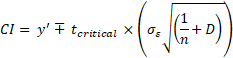
We can use this to compute a confidence interval for the estimated mean response given some value or vector of values, x_p. The linear regression model basically outputs an estimate of the expected value of the response given the independent variables. Here we are assuming that a particular estimation comes from a Gaussian distribution with mean = y’_i and standard deviation = σ_ε. This allows the computation of a confidence interval for our predictions. A confidence interval generally takes the form:

t_critical contains the critical value for the t-distribution at a specific percentage and degrees of freedom (n – 2). The standard error of the fit, σ_f, in this case must take into consideration both the standard error of the estimate, σ_ε, and the overall distance of the given predictor vector from the centre (or mean) of the dataset, X. The latter can be calculated as follows for a single variable:

We can immediately see that the closer the given value, x_p, is to the overall mean the smaller the distance. But this is not the whole story of course, otherwise we could’ve just stopped at the Euclidean distance and be done. The denominator is a sum of distances and it gives us the dispersion of all x values about the overall mean. Large values indicate a noisy dataset widely spread around the mean. This is turn makes it more likely that x_p belongs in the same distribution (assuming normality) and this give us a small distance value. Including this term in the distance means we take into consideration this aspect of the dataset.

For the multiple variable case we need to enlist the help of linear algebra.

 

Incidentally, this equation is also known as the Mahalanobis distance metric with the only difference being that we would take the square root of the term. Here we incorporate the partial covariance matrix of all predictor variables, (X’X)^-1. Any given value in this matrix contains the unique covariance between a particular pair of variables when all other inter-variable covariances have been removed. Like the previous equation this also takes into consideration the dispersion of the points in feature space.  Eliminating this from the equation would basically boil down to a sum of differences between the given vector, x_p, and the mean.

With the distance function on board we are free to provide a decent standard error for our confidence interval for the expected mean value of y’:

This is not the end of the story however. What if we want to know the interval for a specific value of y’? Previously we asked what is the interval for the point estimate E(y’|x_p), now we’re asking what is the prediction interval for the specific, predicted value of y’. The questions are very related but there is a minor difference in the equation:

We add the squared standard error to signify that when estimating the prediction interval there is more added variance proportionate to the degree of deviation of the y values deviate from the regression line.

Assumptions

Before we move on to an example it’s important to bear in mind that one of the strongest assumptions of linear regression is that the data in X are homoscedastic. This means that we expect the same linear relationship between Y and X to hold across the entire dataset. This might not be the case for certain datasets. Take age and income for example. At ages 0 – 18 most individuals would earn a similar amount of money – the regression line would follow a consistent trend in relation to the dependent variable. As people get older though, other things come into play such as education and socioeconomic background leading to vast differences in income across individuals. The linear relationship here would be decidedly different to the one found for the younger group. This spells bad news for linear regression: the nature of the relationship between these two variables is more complex than a humble straight line can describe.

A further assumption is that both the independent variables, X, and the error, ε, are normally distributed which is turn means that y itself is normally distributed (the sum of a set of normal distributed values is also normally distributed). Ultimately, if this assumption holds it makes things easier for us to compute confidence / prediction intervals and infer significance for the model but of course this is not often the case.

Finally we also need to bear to mind the effect of sample size. Generally, the larger the sample the smaller the standard error, the narrower the confidence intervals.  This becomes especially relevant in samples with high variances since small samples will be more susceptible to noise leading to poor fits. Further danger for overfitting is exacerbated with increasing number of parameters. If you only have 25 observations and 10 independent variables you’re effectively guaranteed to overfit even if you do get a very highly significant fit with your training set.

Example

Let’s look at a very simple example. Suppose we have a sample consisting of 500 points of some dependent variable y and independent variable x and we wish to assess their linear relationship.

However, there is always noise during sampling and in real-life scenarios we wish to estimate parameter estimations, b, which best describe the relationship:

The motivation here is to create a model which will allows to predict future values of y given some unseen values of x. 80% of the sample is reserved for training (400 data points) and the rest for testing (100 data points). Here’s what we get for the training set:

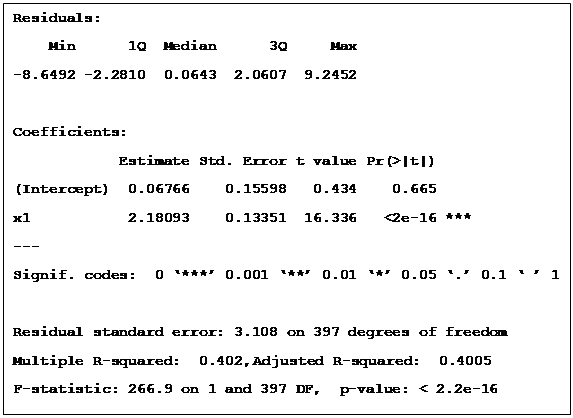
Let’s try and decipher this first. The first thing to notice is that both the coefficient of determination (or R² metric), 0.4, and the F-statistic, 266.9, indicate a significantly good fit between the two variables. But we also realise that just because these metrics are significant does not necessarily mean that there is a true underlying linear relationship. It might just be picking up on outliers or spurrious relationships. So let’s plot the data and have a look.

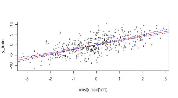
The blue lines indicate the confidence intervals for the slope of the line. They actually look pretty narrow so this at least indicates the confidence of the model in its estimations.

Just by eyeballing the data we can also observe that there does seem to be a rough linear trend between the two and there’s no crazy outliers either.

But how good is the model in predicting new values outside the training sample? One way to assess the prediction performance of the model is by applying the R² metric between the actual values of the testing sample and the predicted values taken from the model. We would expect a strong positive correlation between the two if the model is doing a good job. Correlating the two gives a value of 0.48 which is highly significant (at 98 degrees of freedom). But again it’s good to take a look at a few data points to get a better grasp of the situation.

The red line cutting through the middle indicates where the points should be lined up given a perfect prediction. The error bars indicate the prediction intervals. We can see here that even though the points are pretty close to the lines the intervals are a bit wide.

Let’s add another independent variable to the model. Both variables have means normalised to zero, so the coefficients are comparable. The coefficients are sensitive to the parameters of the variable so it is important to bear this in mind.

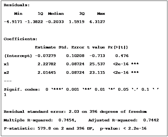
There is an evident increase in the R², from 0.4 to 0.75, meaning that the second variable, x₂, might have a unique contribution to the model’s performance. We can use the Akaiko Information Criterion to get a better handle on whether adding a further variable to our model is preferable to a more parsimonious one (which is less likely to overfit). The AIC provides a unit-less, comparative estimation of how well a model fits the data taking into account the number of parameters. Given two models of equal performance, we would preferably go for the simpler one.

Turns out that for x₁ the AIC score is 2041.25 while for x₁ + x₂ it’s 1702.47. AIC scores are not an exact science but generally the lower the score the better. It means there is a favourable trade-off between model complexity and performance.

There is also a concurrent improvement in prediction performance from 0.48 to 0.74. This validates our initial expectation that this is indeed a very informative variable. Looking at the plot below we also see that the points move closer to the actual value red line and the prediction intervals are smaller.

Suppose now we add a further variable, x₃. How does this affect performance?

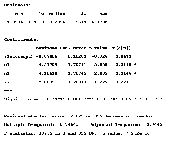
We can see here that there is no noticeable improvement in how well the model fits data. In fact, the AIC score, 1702.952, is a bit higher than for the simpler two-variable model we had before. Prediction performance on the testing set also resulted in a similar R² metric, 0.74. Let’s dig a bit further. Why is this the case?

Looking at the correlation matrix below we see that x₃ is highly correlated with the other variables. This actually makes the variable redundant. In this case we could just drop it and move on with the original ones.

	x1	x2	x3
x1	1	-0.04	0.7
x2		1	0.67
x3			1

This is also reflected in the estimated parameter for x₃ which is in the negative direction. This is because all co-variance between the variable and y has been soaked up by x₁ and x₂ leaving whatever unique variance left.

To wrap this up, it’s worth mentioning that I’ve just covered is the basic, vanilla version of regression. There many other variants which can deal with a variety of datasets. One of the most widely used is logistic regression. Here the predicted variable is categorical and can take 2 or more discrete values. Another useful variant is ridge regression. This is identical in nature to standard linear regression with the simple addition of a penalty term on the number of parameters. It’s particularly useful for prediction because it can significantly reduce overfitting and minimise variance.

In general, all these methods are strongly related in their basic mechanics. Where they differ is how the data is transformed, addition of terms or some other modification.