Language: python 3.5
Code repository: https://github.com/A-V-M/svm_intro

According to Tom Mitchell’s  tome on Machine Learing an algorithm is “said to learn from experience E with respect to some class of tasks, T, and performance measure P if its performance at tasks T, as measured by P improves with experience E“. In the case of classification we want some input, x, to be correctly classified into one of two or more classes, y. Following Mitchell’s aforementioned dictum we need an algorithm which can learn from experience, (input x), attain satisfactory performance (classification accuracy or precision) and generalise well to previously unseen data.

There are a number of methods which try to solve classification problems, each with their own unique approach, assumptions and limitations. Support vector machines (SVMs) have gained a lot of popularity since their general introduction back in the mid 90s. SVMs have been used as a go-to method for classification type problems in industry for image segmentation as well as hand-written digit classification. It is particularly effective in finding linear as well as non-linear decision boundaries for different classification problems. Generally, the algorithm works best with small number of features (relative to the number of training examples) but it can manage pretty well with datasets of large dimensionality. Main weaknesses include long computation times and extensive parameterisation which might necessitate further analyses in the pipeline.

Let’s say we are given a set of two-dimensional feature vectors and asked to classify between two classes. The natural question to ask is what is the best decision boundary for our data? There are a near-infinite number of lines we can pass through the intervening space. SVMs make the clear assumption that the best line is the one which maximises the margin between the classes. In other words, we want a line (or hyperplane in 2 < dimensions) which is as far as possible from either side. And the boundary-defining points of each side are defined as the ones which are bang on the minimum allowed margin from our line.

So, this is what a typical SVM solution looks like. It identified the boundary-defining data points (circled in image) and found the maximum-margin boundary between the two classes.

That’s all good but how did we get to this solution? How do we get w and b?

First, let’s formalise our problem. We wanted a line which best separates our data. How do we define it? We can define a line as:

Drawing this on a 2-dimensional space gives us all the possible solutions which satisfy this equation. w defines the orientation and b the position in relation to the origin. Note that the parameter vector w is perpendicular to the line itself. If a point, x, satisfies this condition then we know it lies on the boundary itself. If the result is larger than 0 then it’s on the positive side of the boundary, if it’s less than 0 then it’s on the negative side. This is now our decision rule.

Now, let’s add a few constraints. First, if we have two classes they’re denoted as y_i = +1 or y_i = -1. Second, I want every sample to have a value indicative of its class:

This allows us to squeeze the above two expressions into one:

If the above happens to give us 0 then we know x lies exactly at margin’s length from the boundary:

As a matter of fact, if we’re not interested in the sign we can re-write this as:

This will come in handy later on.

Next we need to get a handle on the distance for the absolute nearest point x_i to the boundary, otherwise the machinery of the method would break down. In order to do this we need to imagine this line being comprised of some set of points in the feature space. Take any point, x, from this set and then take the vector connecting it with x_i. This gives us the vector x – x_i. Bear in mind that the Euclidean distance between these points – || x – x_i || – isn’t what we want, this is just helping us get there. What we want is the length of the component in the direction of w, in other words the projection of (x – x_i) on w. This is given by:

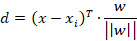
Thankfully we can break this into something simpler. Remember that w^Tx + b = 0 for every point on the plane and that |w^Tx_i + b| = 1 for the closest point to the plain. If we add the constant b from before to both terms on the numerator the whole thing breaks down to:

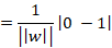
I added the modulus brackets there to show that we want the absolute difference, not really interested in the sign. Now this is the distance we want to maximise. For the sake of making our lives simpler we inverse this to ||w||² / 2.

Ultimately this becomes an optimisation problem with the objective to minimise ||w||² / 2 with the constraint y_i (w^Tx_i + b) – 1 = 0. This gives rise to the following Lagrangian:

Differentiating with respect to w gives us:

When this expression equals to zero then we get the following:

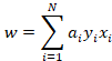
Here we find to our delight that w is nothing more than a weighted linear combination of our feature vectors.

We differentiate next with respect to b:

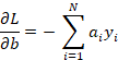
Again when we are at the function’s minimum we get:

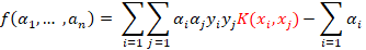
Assuming then that both these differentiation functions are at zero we can plug them in the initial Lagrangian to get:

This is known as the dual formalisation of the problem. The parameters we enter here are our sample feature vectors. We minimise with respect to a subject to the constraint that all a‘s are equal or greater than zero. The vast majority of the sample points will have a = 0 – the only exceptions will be the support vectors, i.e. the points closest to the decision boundary hyperplane.

It’s important to notice the highlighted terms. You see at the core of the method’s machinery lies the simple and familiar dot product. And this becomes very (one might even say, infinitely) useful when we are faced with hairier problems than the simple example presented here.

So now we solve the optimisation (typically quadratic programming comes into play here), extract the values for the α’s and get the all-important w.

We then plug them in the hyperplane equation (w^Tx + b = 0) and solve for b assuming x are the point coordinates of our support vectors. We know the support vectors from all a > 0.

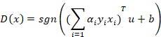
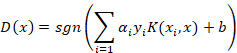
Below we get the decision function, over the test set, for some point u in terms of a and b. We are only interested in the sign, the real value is not important.

As an initial sanity-check of the decision function we can also enter the point coordinates of our support vectors and hopefully it’ll give us 1 (the minimum absolute distance allowed from the boundary).

And I guess that’s it.

Or is it?

Unfortunately the world isn’t this simple. The hard-margin approach described above works perfectly if our dataset is linearly separable and non-overlapping. But what happens if these assumptions are violated?

Soft-margin SVMs

Let’s stick around with the linear case first. There might be some linear boundary but unfortunately it is obscured by our noise-riddled data. In other words there is overlap between the two classes making a clear-cut linear boundary in the feature space intractable. This makes things rather foggy for our classifier.

The constraint we imposed for the hard-margin case, y_i (w^Tx_i + b) ≥ 1, is impossible to satisfy here for all training samples. Any computed hyperplane will inevitably produce classification errors during the training phase. So we have to compromise with maximising our margin between classes on the one hand and minimising training error on the other.

We have no choice but to allow the decision boundary to misclassifiy some samples during training but we need to keep track of the error. This error is quantified by ζ_i.

 

For samples which are on the correct side of the hyperplane but on the wrong side of the margin then 0 < ζ_i < 1.

For samples which are on the wrong side of the hyperplane and on the wrong side of the margin then  ζ_i > 1.

The only case where ζ_i = 0 is when the sample satisfies our original constraint.

We now formulate a new constraint which takes the error into consideration:

This creates an issue for us however. Just trying to minimise ||w|| is not going to cut it anymore. If we do that then we are giving the optimisation process free rein to maximise the margin with complete disregard of the training errors. For this reason we incorporate errors into a new objective function for the classifier:

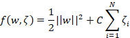
The right part measures the overall error (or loss) with C being the scaling factor and the other is the squared norm of w. C is a free parameter and it defines how much penalty we are going to apply to the errors. (As a side-note this function can be implementation-dependent. Scikit-learn implicitly uses this but there’s always the possibility that other packages might have the C parameter on the margin term. In that case, increasing C will have the opposite effects to the ones described below)

The dual formalisation for the Lagrangian is the same as before with the difference that values for a have an upper found at C. Samples with a = C will be ones on the wrong side of the margin. This in turn increases the complexity of the model.

So what happens when we put this function through an optimisation process? As we explore the parameter space we find that large values for C will force a severe penalty on misclassified terms. Concurrently, the decision boundary will try to accommodate for as many training samples as possible sacrificing margin width (1 / ||w||) in the process.

But of course there’s a caveat. As C tends towards infinity it behaves more and more like a hard-margin SVM, the margin becomes too small and generalisation power is reduced due to overfitting. In a way we are being excessively sensitive to errors during training and not allowing the classifier to “loosen” up its assumptions when faced with new data points. This becomes particularly problematic when there’s outliers in the data which might skew the boundary in non-optimal directions.

On the other hand, if C gets too small then the margin becomes large, training errors have little effect on the decision boundary and ultimately the model is not sufficiently representative of the true underlying pattern which separates the two classes. In fact, even in perfectly separable cases the margin can grow large enough to include a substantial portion of the dataset.

Soft-margin SVMs: First example

We have two different classes of data, one in blue, the other in red in the images below, drawn from different distributions. I use a SVM to separate between the two using 80-20 cross-validation split.

So here there’s no clear-cut linear boundary. At low C values the margin is quite large meaning it does great during training (even though there’s only two blue points left in the blue category!) but not too well during testing (accuracy = 0.775). As a matter of fact, precision and recall will be much worse. With increasing values of C we get to a point where the margin is sufficiently wide to allow for an acceptable training error and sufficiently narrow to achieve near-ceiling accuracy during testing.

Soft-margin SVMs: Second example

Now let’s look at another example where there’s more noise leading to further overlap between classes:

So here it looks like the C parameter hits an optimal value around 0.1. Increasing it further leads to no noticeable change in accuracy, be it negative or positive. Why is this the case? Intuitively, we can interpret this as being in a situation where the data pattern is too complex for a linear solution. Therefore overfitting is unlikely in this case since the ceiling training accuracy is far below 1 – the paradigm itself is too simple to account for the subtle differences between the two classes.

Non-linear SVMs

Now what about the non-linear case? This is where the SVMs truly show their hidden power. Because it turns out the mathematics behind SVMs allow the seamless transformation between higher (or even infinite) dimensional spaces by means of the kernel trick. Note that ultimately the dot product is a measure of similarity, high values indicate that vectors are in similar directions, zero means they are orthogonal to each other. The kernel allows us to get the dot product of two features in a transformed feature space without going through the hassle of computing the actual feature transformations. This particular incarnation of SVMs is an example of a non-parametric classifier: the kernel itself discards the distributional parameters of the features. In fact, the parameters in the newly transformed feature space could be potentially infinite. Linear SVMs are parametric models: classification is fundamentally dependent on parameters w and b.

A kernel here is simply a stand-in function instead of the traditional dot product. In fact, the kernel computes the dot product in a different feature space where a linear boundary is more tractable. There are two functions where the kernel is explicitly involved. When computing the α’s:

And for the decision function:

A widely-used kernel is the Gaussian radial basis function calculated with the following equation:

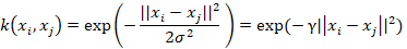
The Gaussian RBF is a non-linear kernel which measures similarity as a function of both the squared absolute difference and the variance. The free parameter, γ, is inversely proportional to the degree of influence exerted by variance on the similarity. Low γ translates to high variance in computing the kernel and vice versa. We can think of γ as defining the radius of a sphere around a point. Anything falling into this sphere is granted a shared category membership. You can imagine a wide sphere (i.e. low γ) as absorbing neighbouring points, brushing over their unique position in the feature space. This is good if our data is centred around the class mean and classes are well separated. But if this is not the case then we have a problem. We need to shrink down the sphere until it can accommodate the idiosyncratic arrangement of the points in space.

An increase in γ will lead to a decrease in the computed similarity between any two given points. When applying this to the decision function this means that even neighbouring data points to the support vectors will score low similarity leading to increased testing error (i.e. the model suffers from overfitting). At the opposite end of the spectrum, exceedingly low γ values lead to increased similarity which blurs over the complex arrangement of data points in the feature space. This leads to a simple (and underfit) model which may resemble a solution provided by a linear kernel.

Non-linear SVMs: Example

For the following example, there is a clear trend from an underfit model at γ = 0.001 to an overfit model at γ = 100. At low γ the boundary is too simple to provide decent separation hence low accuracy. As γ increases we reach a point where the model is overly sensitive to individual data points and again the model suffers from a poor accuracy score.

With a decent optimisation procedure to pinpoint a good set of tuning parameters SVMs are a solid first line of attack for most classification problems. One thing to note is that due to the way the margin is calculated, SVMs are particularly sensitive to scaling so this is definitely something to be aware of during data preparation. However, the method is less sensitive to the distribution of the data and less demanding of normality especially compared to conventional linear methods (etc regression). This is largely because the margin is dependent on the support vectors with no bearing on the interior data points.