Language: Octave 4.2.1
Code repository: https://git.io/vbes0

Everything in nature belies some hidden, underlying structure; a universal regularity which scaffolds the individual instances. Over the course of analysing data, we are trying to capture some sense of this structure based on a collection of observations.

Let’s take faces for example. We’ve all come across a myriad of different faces each with their own unique characteristics. But looking beyond the fine-grained details, some regular patterns emerge across the entire population. The positioning of the eyes and nose for example and the distances between them, the height and width of the forehead etc. In other words, there are certain dimensions along which we can describe any face we encounter in the environment.

The question now is how do we unravel these hidden dimensions? If there are many, how do we quantify their importance or relevance? This is perhaps the prime motivation behind statistical procedures such as principal component analysis (PCA), to take some data with no prior knowledge of their classes and produce a new feature space which allows us to gain insight into its internal structure.

PCA has been around for more than a hundred years now since famed polymath Karl Pearson published a paper introducing the method in 1901. Since then it has been used heavily, under different names and for various purposes, in fields ranging from mechanical engineering to neuroscience.

So how does it work?

Much like mostly everything in statistics, the roots of the method lie in linear algebra (which brings along with it its own assumptions and biases). So let’s say we have an m x n matrix M. Each column, n_i, is a feature and each of the rows, m_i, is a specific instance. Before we proceed it’s important to make sure that the units of measurement are the same across all rows. It’s standard to substract the mean from each row thus squashing all means to zero. Most importantly, this procedure ensures differences in mean scores between observations won’t influence how the principal components are formed.

M is a non-square matrix which means it’s not full rank, i.e. many of its columns (or features) will be linearly dependent. The next step is to quantify how all these features co-vary with each other. Covariance between two variables for a given sample is formally defined as:

Notice the degrees of freedom here (n-1) since we typically assume that our data comes from a small sample and not the entire population. When we are dealing with many variables (as columns of a matrix) we can represent this set of operations more concisely as the cross-product of M with its transpose and ignore the constant denominator:

We now end up with a square matrix of dimensions m × m, where each element V_i,j contains a value proportional to the true covariance between features i and j. But how exactly can we extract any useful information from this matrix beyond its elements? Are there any specific properties which might provide us with some insight regarding our data?

It turns out that there are but first we need to appreciate what are eigenvectors and eigenvalues. Let’s take a vector, x, and a value, λ, are such that Ax = λx. x in this case is said to be an eigenvector of A while λ is the corresponding eigenvalue. An eigenvector has the unique property of remaining unchanged, i.e. it does not change direction, even after we apply the transformation matrix A. The only change is the scale which is quantified by the eigenvalue.

Going back to the covariance matrix, we can decompose it into a set of eigenvectors. These eigenvectors would then represent unique directions of variance of the dataset. The corresponding eigenvalues denote the amount of variance each eigenvector captures. To get a sense of proportion we divide each eigenvalue by the sum of all eigenvalues.

Getting the eigenvectors

Although at least on paper decomposing the covariance matrix is the most straightforward way to extract the eigenvectors, oftentimes this process is computationally costly. Singular value decomposition (SVD) is an alternative way which reduces processing demands and produces the same results. Our starting point here is the initial matrix M which is decomposed, by a process which is beyond the scope of this post, into the following:

U is an m × m matrix (m is the number of samples) containing the extracted eigenvectors for MM^T, V is a n × n matrix (n is the number of features) containing the eigenvectors for M^TM (V* is the transpose of V) and Σ is an n × m rectangular diagonal matrix which contains the eigenvalues.

It is very important to highlight the shape of the matrix, M. I am assuming that the rows are samples, m, and the columns are features, n. If it were the other way around, i.e. n × m instead of m × n, then we’d have U being the left singular values, n × n, containing the eigenvectors for M^TM and V the right singular values, m × m containing the eigenvectors for MM^T.

V and U are related in the following manner:

Where k denotes the k-th eigenvector. Elements in U_k denote how “aligned” a particular sample is to the direction of the principal component. Eigenvectors in V are basically linear summations of all samples weighted by eigenvectors in U normalised to unit length. Values in V_k are the coefficients for each variable in our dataset. It tells us how related the k-th eigenvector is to each variable. These values are also known as the loadings of the principal componets.

Projecting data into a new subspace

We can now project our samples from the original data, M, to a new subspace spanned by the eigenvectors. What we are interested in is V from the decomposition above.

Where E_k is the rank-k approximation of vector X_n. A_k is the n × n outer product matrix between V_k and V_k’. This process guarantees that the best rank-k approximations are afforded by the first k eigenvectors (in order of magnitude of their eigenvalues).

Computing the scores

The rank-k approximation, E_k, of a vector X_n is a linear combination of k eigenvectors. What we don’t know is the contribution of each eigenvector, e. These are known as the scores. We could attempt a linear least squares approximate solution. First let’s formalise the problem:

Notice that the approximation E_k is effectively a function of X_n. So let’s go ahead and replace it:

We then multiply each side with the transpose of V_k, a familiar first step when finding an approximation for our parameters in a different subspace. I’ve also expanded A_k as an outer product of the eigenvectors. This will become useful later on.

We know that V_k contains a set of vectors which are orthogonal to each other and unit length. This makes things a lot cleaner since the product of such matrices, V_k’V_k, is the identity matrix (diagonal of 1’s with all other elements being zero). I can just remove it from the previous expression then only to be left with:

e is a k × 1 vector containing the scores for each of the k eigenvectors. This equation tells us that the score for a particular principal component (or dimension or eigenvector or whatever you want to call it) is the dot product between the eigenvector  (or loadings) in question and the original sample vector. We can interpret this as a weighted sum. The singular values in V are like coefficients. If a particular feature is deemed important in explaining variance along that component then it will carry a high weight. Samples in our dataset which have highly-weighted features will score highly overall in the direction of that component. This way we are compressing a lot of information into a single-value summary.

Example: Reducing face images to a lower-dimensional space

Now we are ready to consider our initial example – human faces. I collected an image dataset from the Olivetti Research Laboratory (known as Database of Faces).

We can formalise an instance of a face in the form of a p × j matrix. Each element in our matrix denotes the pixel intensity at that particular location (for the sake of simplicity let’s assume it’s monochromatic so we only need to care about one value per pixel). We then convert this matrix to a column vector of size (p × j) × 1.

If we keep doing this for all images in our set we’ll eventually end with an m × n matrix M. We then apply SVD on M to get the eigenvectors and eigenvalues in V and Σ respectively. The bar chart below shows the proportion of variance each eigenvector captures as quantified along the sum-normalised diagonals of Σ. To save some space I’ve only included the top 10.

In the field of face processing, these eigenvectors are generally known as eigenfaces.

These are the top 9 eigenvectors or eigenfaces.

The original face dataset can be represented as a linear combination of eigenfaces. The scores of separate images on a subset of these can also allow for low-dimensional codings.

Now let’s project our images to new rank-k subspaces:

Notice that the first principal component is not really very informative even though it accounts for most of the variance in the set of eigenvectors. It seems like it’s sensitive to very broad facial features like forehead, overall shape etc. As we add more PCs to the subspace, more detail begins to appear. Eventually, at n = 353 the image is almost indistinguishable from the original. This is also reflected in the monotonic decrease in reconstruction error across all images in the set.

Let’s add some noise to the image. A 5 × 5 Gaussian kernel (σ = 1.5) is applied to remove some detail from the image. I also added Gaussian noise (μ = 0, σ = 45.96; same as the image’s parameters) to another copy of the same image.

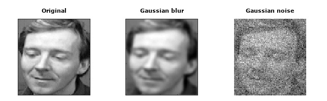
Reconstructing image from original image plus Gaussian blur.

Reconstructing image from original image plus Gaussian noise.

Let’s have a look at the reconstruction errors.

Apparently, the PCs do a good job at reconstruction here. This suggests that the eigenvectors can abstract away from individual, fine-grained details and pick up on regularities across different faces. This is probably why blurring doesn’t really affect reconstruction – the general features are retained.

Now let’s see how well these new dimensions do in separating between different individuals. First, we compute the PC scores for each image. Below, I’ve picked two random individuals and plotted the scores for each of their face-images. Looks like even with just two dimensions we’re doing a decent job separating between individuals, at least for these specific ones.

 

Interestingly enough it seems that categories are very well separated even when using just the first two PCs. This is a good thing to know when compressing images. We can still extract a fair deal of general information even when we compress images to just two dimensions.

So there you have it. PCA is a powerful technique for feature transformation, dimensionality reduction, data exploration etc. However, there are certain caveats to keep in mind:

1. It’s generally good practice to transform your data if it’s heavily skewed, non-Gaussian (e.g. log-transform).
2. Doesn’t work well when you have more instances than features.
3. In some cases it might be completely inappropriate. For example if we want to disentangle a signal buried in noise/other signals it might be best to use Independent Component Analysis.