Language: Python 3.5
Packages: scikit-learn, nltk, Beautiful Soup, seaborn, slimit
Methods: clustering, text processing
Code repository: https://git.io/vhLsz

Approximately 80% of data on the web is termed as “unstructured”. What this means is that there is a good number of terabytes worth of unprocessed, unwieldy raw information floating out there, never intended for analysis in the first place. This sort of data poses a unique set of challenges quite distinct from conventional approaches which assume the explicit use of data models where information is neatly arranged into a structure and ready for analysis.

It’s a state of affairs which is quite reminiscent of the type of questions one is faced in academic research. Nature doesn’t bother with conforming to our formalisations and descriptive conventions. And I’m afraid it’s a truth that any person who seriously deals with data on a regular basis must accept. Although in our naivety we rush to employ our favourite classification technique the big challenge many a time is sorting out what can be analysed from the noise. In fact, and I must admit that this was a recent revelation to me, unsupervised learning will see a steep rise in popularity in the coming years as we steadily become more and more flooded with messy data.

This is my first real foray into web scraping. Unlike previous projects here there’s no clear hypothesis to be tested, no objective function to be minimised, no performance metric to be evaluated. I’m just exploring the surface with a flashlight and hoping that something interesting comes up.

The whole endeavour is split into 4 parts, first scraping the necessary data, cleaning it up, formatting it into a structure which we can use and finally some rudimentary exploration.

Data scraping

I wrote the scraper in python using packages Beautiful Soup 4.6.0 for parsing in the HTML code, newspaper for text extraction and slimit 0.8.1 for handling JavaScript. The intention of the script was to collect job descriptions from online job advertisement website, indeed.com (raw data pickle can be found here). The pages were coded in both HTML and JavaScript which I had to query accordingly. I managed to collect a total of 1016 job descriptions (up until May, 2018) which were then used in the next stages of the pipeline.

Data cleaning and formatting

Standard document processing starts with transmuting the raw text into a representation which we can operate upon. For my case I used a vector representation where elements are linked to specific tokens found in the document. Tokens in this case were bigrams and unigrams. What do the elements denote? We could just have a binary vector indicating the absence of a particular token. But that’s missing out a lot of information. The most common formalisation is the term frequency-inverse document frequency (td-idf) measure which is the one I used. It takes into consideration both the number of times a token occurs in a document balanced by its overall occurrence across the entire corpus.

All punctuation and stop-words were removed, and text converted to lower case. Considering that ‘R’ and ‘C++’ case-sensitive terms with the latter also including punctuation these were exempted from the transformation.

Certain tag combinations in the case of bigrams were also removed from the final document-word matrix. Tags refer to the word type (e.g. particles, noun, adjectives etc). Combinations between particles and conjunctions for example; such as “and this”, “or that” had to be removed since they convey little information regarding the document’s specific content.

There were also peculiarities specific to the data itself. Every description was appended with advertisements and recommendations for other jobs. Thankfully, they were prefixed by a consistent sequence of words which allowed me to detect them easily during processing and remove them.

Finally, given the nature of the data source there’s a good chance that certain job descriptions might appear more than once in the listings. Duplicates were defined as documents with a cosine distance of zero between their corresponding vectors. Removing these, resulted in a 851-document by 94561-token matrix.

Data exploration

Word salience

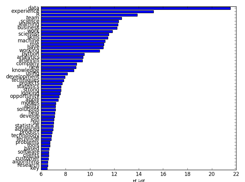
The naturally first question to ask is word salience. Which are the most important words across the entire corpus? To do this I calculated the weighted sum of occurrences across the documents. The weight here is simply the td-idf for a particular word found in a particular document. Below are the top-15 ranked unigrams (1-word tokens).

And of course the bigrams as well:

Unsurprisingly the top words that come up are data-centric. Apart from ‘R’ and ‘python’, there are no terms or words directly relevant to data science which come up. The corpus is denominated by action words (e.g. ‘experience in’, ‘working with’, ‘are looking’) which are predominant in most job descriptions of any kind.

Word co-occurrence

Certain words can co-occur together which can provide a sense of context for the word’s actual meaning. K-means clustering is a good first approach to see if there’s any underlying clusters – it’s fast with easily interpretable results. However since I’m only interested in co-occurrence I used the binarized version of the matrix. Here elements simply denote the absence/presence of a token and nothing else. I also had to code a custom-made version of k-means to deal with binary data. I tested for k = [1,10] with the mean entropy across conditional probabilities as my cost metric (for more information on this method you can check out my github repository).

I used multidimensional scaling to reduce my dataset to two dimensions and get a sense of any glaring patterns. Size of the points is proportional to their word salience score and the color signifies the cluster they belong to.

 

There is a tight, ‘hub’-like cluster of salient, highly co-occuring tokens including ‘machine learning’, ‘experience’, ‘data’ and ‘python’. For single words it’s clear that their high salience is because of being tagged along with certain bigrams which are more contextually relevant. For example, ‘learning’ is used in conjunction with ‘machine learning’ and ‘science’ with ‘data science’ or ‘computer science‘.

We can imagine single words like roots of a tree, where branches denote the different combinations which can be formed. Below are the most similar tokens to each of 5 selected words.

Experience: [‘and experience’ ‘experience in’ ‘experience of’ ‘experience with’ ‘experience working’]

Scientist: [‘data scientist’ ‘data scientists’ ‘scientist to’ ‘scientists’ ‘scientists and’ ‘scientists to’]

Science: [‘computer science’ ‘data science’ ‘science and’ ‘science or’ ‘science team’]

Machine: [‘and machine’ ‘development machine’ ‘machine learning’ ‘of machine’ ‘or machine’ ‘python machine’]

Lead: [‘leading’ ‘to lead’]

Ability: [‘ability to’ ‘capability’ ‘the ability’]

We can see that the word ‘machine’ tends to be found in bigrams such as ‘machine learning’ and ‘python machine’,  the word ‘scientist’ most often refers to data scientists or it’s attached to pronouns which add little to its unique meaning. We could potentially add another step during the pre-processing stage and collapse all these words into one group representative of the word’s contextual meaning. For example, tokens ‘ability’, ‘ability to’ and ‘the ability’ could all be merged under a single vector and economise space for the feature matrix.

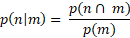
I’m also personally interested in whether certain programming languages are probabilistically tied to specific tokens. Are certain words predictive of ‘python’ let’s say or ‘R’?

Assuming binary vector for words w_n and w_m conditional probability of finding word n in a document given another word m is here defined as:

First thing to notice is that technical terms such as ‘algorithms’ and ‘machine learning’ are highly predictive of python, R and C++. Excel on the other hand seems like a bit of an outlier being mostly associated with terms like ‘business’ which is understandable given that it’s not really a language and typically used in tasks which are quite distinct from the ones typical of more technical languages. An important thing to note here is that sql is the only language to appear in the top-15 of three other languages – ‘python’, ‘matlab’ and ‘excel’. This highlights the widespread use of SQL in various contexts.

Document clustering

For this section I asked whether there are specific types of jobs that might be characterised by a strong emphasis on specific skills / programming languages academic background.

I used non-negative matrix factorisation for clustering. Like other factorisation techniques it “breaks down” a given matrix V into two matrices W (documents by clusters) and H (clusters by words) such that V ≈ WH. The factorisation is approximated through an iterative process (I used the multiplicative update rule) until W and H reach stable values. We can extract cluster weightings (or scores in PCA lingo) for a specific data point (or document) d by the dot product Wd.

NMF is parameterised by the number of clusters and the type of error function used to estimate the distance between V and the reconstructed matrix V’. For number of clusters I fitted the model for n = [2,10]. There was a very minor increase in performance with a serious increase in processing time and so I opted to go for just two clusters which would also allow me to visualise the results.

I used the standard Frobenius norm as my error function (a variation of the familiar Euclidean distance).  The following bar plot shows the two clusters (or topics) extracted using this method with the top-10 words.

‘data’, ‘experience’ and ‘R’ figure in the top for both topics with ‘learning’ and ‘work’ also featuring in the top-10. The most distinguishing words are ‘business’ for topic 1 and ‘science’ for topic 2. We might say there is very vague distinction between more business-oriented job descriptions and science-based roles but it’s obvious that there is very little variation across the entire corpus of documents. This also explains why increasing the number of clusters did not confer any substantial improvements in reconstruction performance. In fact, it’s plausible to collapse the entire corpus into just one ‘summary’ cluster.

I plotted the documents using the calculated scores. It’s important to note that scores cannot be negative in NMF (as the name might suggest). There are negative values on both axis on the plots purely I centralised the values by their respective medians. The length of the arrows denote the weight those particular words carry. We can see below that R and python are the two strongest languages which determine the most typical of job descriptions for data science. As expected there are no strong weights which might be orthogonal to each other – most point to the same direction. Similarly, ‘machine learning’ and ‘statistics’ are very important.

It will also be nice to have a sense of the distribution of the values across these components. Kernel density estimation provides a non-parametric way to estimate a distribution probability density function. It achieves this by smoothing individual data points with a kernel (in this case the Gaussian kernel). The spread of the curve is dependent on the bandwidth – small bandwidths mean shorter spreads. The bandwidth was determined using the Scott estimate (as coded in seaborn 0.8.1). We can see that most of the documents clusters around the median values with a very small number of outliers across the nether-regions of the space.

Conclusions

Data science jobs are quite consistent in their descriptions. There is a core cluster of terms, ‘R’, ‘experience’ and ‘machine learning’ which appear consistently and prevent any discernible variability across documents. Further work might include segmenting by city or including additional variables such as salary and precise job titles (junior vs. senior).