
Language: Python 2.7
Packages: scikit-learn, nltk
Methods: random forests, support vector machines, latent Dirichlet allocation
Code repository: https://git.io/v5QfT
Introduction
Spam detection remains one of the most widely used applications of machine learning. Building algorithms which can effectively detect spam, or any other type of text written with an intent to deceive, is especially relevant when we take into consideration how today’s users form opinions about anything, from household appliances to finding accommodation. Generally, humans are quite susceptible to deception particularly within the written media and only marginally perform better than chance (Ott et al., 2013). This is turn allows certain individuals to easily find ways in writing up convincing feedback and reviews to skew the true, general opinion for a product or service. Detecting fraudulent behaviour such as this then becomes crucial both in protecting the consumer from deception as well as the validity of said online ratings and reviews.
For this project, I will be addressing a particular form of deception which is quite prevalent on sites featuring user-generated reviews for various establishments in the service industry (Jindal and Liu, 2008). Websites such as TripAdvisor and yelp.com are a standard resource for people wanting a reliable and objective opinion of their establishment of interest. And although this is mostly the case there are cases which have been put there with the clear intent to deceive
In developing this project I will be focusing on hotel reviews. Specifically, the prime objective is to construct a classifier which can predict, with a reliable degree of accuracy and precision, whether a given review is fraudulent or not. Accuracy is the most intuitive metric and simply refers to the proportion of correct predictions the classifier has made: where TP refers to the number of true positive, TN the number of true negatives and T that total number of predictions. Precision, or otherwise known as positive predictive value refers to the proportion of true positives made over the total number of predicted positives: . It informs us of how likely a condition is an actual positive given a positive prediction. To achieve an acceptable performance it is very important to provide the classifier with an appropriate set of features. Previous attempts by Ott et al (2011) have resorted to techniques based on theoretically derived parameters as well as strictly text based features (i.e. n-grams). They managed to achieve a high accuracy (89.6%) with the methods at their disposal but, given the developments in text processing there is good reason to believe that better performances can be attained.
The project will be carried out through a two-stage pipeline. For the first stage, I intend to extract classification-relevant features from the text dataset through the use of a technique known as topic modelling (explained later). For the second stage a set of classifiers will be trained on the features from the previous stage. Finally, the classification performance will be assessed and presented.
Topic models
Topic models belong to the broad family of generative models. Their usage is not strictly confined to text processing since they have been applied to fields such as genomics, images and networks (Blei, 2012). They can be considered an unsupervised learning method since the ultimate aim is to extract latent features which might provide some insight into the underlying structure of the data in the absence of labels (as in the case of supervised learning). In the context of the project, I am using them as a pre-processing tool to reduce dimensionality and increase classification performance.
The most common type of topic model is latent Dirichlet allocation (LDA). The central assumption under this model is that documents are comprised of a small number of topics being drawn from a prior Dirichlet distribution. Topics themselves are comprised of a small number of words which are probabilistically interlinked.

The plate notation above illustrates how prior parameters (α, β) influence the building blocks of a document, words ![]() and topics (Z). M is the number of documents and N the number of words. Adapted from Wikipedia Commons.
and topics (Z). M is the number of documents and N the number of words. Adapted from Wikipedia Commons.
The formal definition of a topic, under LDA, is a probability distribution over words (φ in the above diagram). Elements in the topic will denote a probability attached to a certain word. For example in a “biology-topic”, words such as cell, genome, respiration will have a high probability attached to them. Documents in turn are defined as a distribution of topics (θ in the above diagram). The overarching purpose is to find a set of topics which maximise the likelihood of a particular document.
Analysis
Data
The data for this project was originally acquired by Ott et al (2011) and made available via the Kaggle© competition platform (https://www.kaggle.com/rtatman/deceptive-opinion-spam-corpus). It comprises of a total of 1600 entries broken down into 800 deceptive and 800 truthful reviews. Each set, deceptive and truthful, was further broken down into positive and negative reviews. According to the researchers carrying out the original study, deceptive reviews were collected by having volunteers intentionally writing up and posting reviews on various websites while truthful reviews were harvested, non-modified in any way, from TripAdvisor. Both sets were matched for document length and normalised to unit-length (for both negative and positive reviews) before further processing.
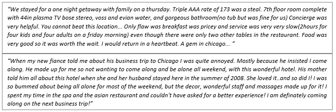
Below is a sample pair of reviews. The top one is a positive genuine review while the bottom is a positive deceptive one.
The aim of the project will be to improve upon the performance reported by Ott et al and thus increase the capacity to detect deceptive reviews. I intend to do this by focusing firstly on the informational quality of the features used. Classifier performance is highly dependent on the training features set they’re operating on. For this reason, I’ve chosen topic modelling which allows one to distil the “essence” of a document to a few thematic topics thus abstracting away from the words in isolation and give rise to a more concise, formalised representation. My reasoning is that it is this additional step which will improve classifier performance. Following on this, the choice of classifier will not deviate vastly from the ones used in the original study. I will be utilising both SVMs (which produced the best results for the original study) and random forests.
Design
In both the present and previous studies (Ott et al, 2011) the main evaluation metric is classification performance. Within the context of the present project, the main difference will be the type of features used for the classification. The standard, go-to method is to break down a document into a list of n-grams and then perform classification on the corresponding document’s tf-idf vector (term frequency-inverse document frequency). Ott et al did exactly that and had significant success with the bigram feature set (i.e. the resulting list comprised of all possible two-word combinations found in the documents). Given, the relative popularity of this document processing procedure as well as the satisfactory performance for the study I will be using this as my benchmark model with SVMs as the standard classifier.
As mentioned in the Background section, I will be using a method known as topic modelling during the feature extraction stage of the pipeline. Topic modelling is generally used as an unsupervised method (Steyvers and Griffiths, 2007; Blei and Lafferty, 2009). It “digests” a set of documents (known as a corpus) and reduces it to a set of a predefined number of topics. Any given document can then be described as a distribution over the extracted topics. These topics are effectively a “summary” of the main themes that a document might be about. The method has found considerable success, in and of itself, when applied to document classification tasks (Blei and Lafferty, 2007) but for the purposes of this project I shall attempt to utilise its output as a substrate for an additional, classification, stage.
The classification stage itself will be comprised of two methods: SVMs and random forests. The former is included to have a level plain-field with the previous study (who also used SVMs) and the latter to explore whether overall performance could be improved further by using an alternate classifier. Given that a priori knowledge regarding the features which the classifier will be trained on is impossible before the first stage takes place, it is important to utilise an appropriate algorithm that has minimal assumptions about the training set. Random forests deal quite well with noisy, non-linear datasets and are less likely to overfit compared to more conventionally and closely related algorithms such as decision trees.
Preliminary visualisations and word analysis
Before embarking on the classification training and testing I decided to first analyse the distribution of words across and within the two different categories (deceptive vs. authentic). It is conceivable that a more parsimonious and tractable solution to the problem should be disqualified first before moving on to more complex approaches. I also expected that this analysis would provide useful insight when interpreting the results of the classification stage.
There were three parts taken for this stage:
- word frequencies within each category (do certain words appear more frequently in a particular category?),
- word type distribution within each category (do certain types of words more prevalent in a particular category?),
- word information. (which are the most informative words (in bits) with regards to category membership?)
Word frequencies were calculated across the entire text for a particular category. I merged all reviews (for either truthful or deceptive) into one document and then extracted frequencies for all individual words.
Word types were extracted using the Natural Language Toolkit (as implemented in Python 2.7) which recognises a total of 33 types or tags such as pronouns, prepositions, numerals etc. As with word frequencies I merged all reviews into one document and then assigned a tag to each word. Following this, I calculated the frequency for each assigned tag for each category.
Word information is closely related to the probabilistic relationship between individual words and categories. Mutual information in this sense refers to how much information we gain about whether a review is deceptive or authentic by knowing the occurrence of particular word. Mutual information was calculated by using the following formula:

One could also argue that the higher the information gain of a particular word the more relevant it is during classification. To calculate information gain as a percentage, I carried out the following operation:

In order to visualise the word frequencies for each respective category I decided to use a word cloud depicted below (using WordCloud 0.18). It can be observed that, unsurprisingly, both categories have a high prevalence for “hotel” and “room”. “chicago” is a word seemingly more prevalent for the truthful reviews which is quite interesting in and of itself since it would appear that reviews written with an authentic intent refer to locations and spatial descriptions.

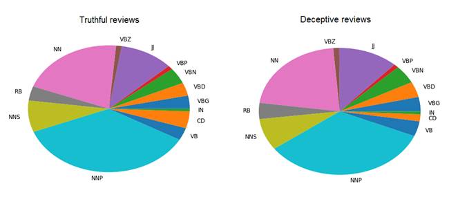
Word types did not appear distinctly different between categories. To avoid visual clutter I only counted types which appeared more than 50 times in the respective category.
| CC: conjunction, coordinating | CD: numeral, cardinal | DT: determiner | EX: existential there | IN: preposition or conjunction, subordinating |
| JJ: adjective or numeral, ordinal | JJR: adjective, comparative | JJS: adjective, superlative | LS: list item marker | MD: modal auxiliary |
| NN: noun, common, singular or mass | NNP: noun, proper, singular | NNS: noun, common, plural | PDT: pre-determiner | POS: genitive marker |
| PRP: pronoun, personal | PRP$: pronoun, possessive | RB: adverb | RBR: adverb, comparative | RBS: adverb, superlative |
| RP: particle | TO: “to” as preposition or infinitive marker | UH: interjection | VB: verb, base form | VBD: verb, past tense |
| VBG: verb, present participle or gerund | VBN: verb, past participle | VBP: verb, present tense, not 3rd person singular | VBZ: verb, present tense, 3rd person singular | WDT: WH-determiner |
| WP: WH-pronoun | WRB: Wh-adverb |
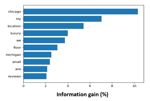
Finally I looked at the information content of individual words. Words which appeared less than 50 times were not included. This was because, words with such low frequency might incidentally occur in only one document. This would lead to words scoring high on mutual information even though they are unlikely to appear in documents outside the corpus. In addition, common words such as at, the, for were not included since they are quite ubiquitous and unlikely to be informative of any one particular category. It appears that the most informative words are location-based (“Chicago”, “Michigan”) or even more abstract such as “location” and “ave” (short for avenue).
In summation, the word analysis did not reveal noticeable differences between words or word types. There were however interesting regularities when observing word information specifically with respect to location-centric words.
Benchmark model
The initial study reported a peak performance with the use of SVMs as the classifier of choice and bigrams as the document tokens. Bigrams here refers to sequential two-word combinations. For example in the sentence, “the cat sat on the mat” the extracted bigrams would be “the cat”, “cat sat”, “sat on”, “on the”, “the mat”. Bigrams can provide context and thus more information when compared to single words. I carried out a 80-20 split for the training and testing sets respectively. This meant the classifier was trained on 1280 documents comprised of 83000 features using 5-fold cross-validation and tested on the 320 remaining documents. All features were normalised to unit length.
Parameter optimisation was carried out using a gridsearch method. The parameter set used was kernel type (linear, radial basis function), C ([0.1,0.4,1,10,100]) and gamma ([0.001, 0.0316, 1, 31.6, 1000]). Kernel type here refers to the function used to transform features. A linear kernel will typically assume that the data is linearly separable and try to find a pair of hyperplanes which maximally separate the two sets. It will try to maximise the margin between the two hyperplanes via an optimisation process. The C parameter controls the size of this margin with respect to how tolerant we want the classifier when misidentifying positive cases. A large C value will lead to small margins which in turn leads to a lower chance of false tests but a higher chance of overfitting. A radial basis function on the other hand is more flexible in the sense that it can find sensible classification boundaries in cases where the data is non-linearly separable. It achieves this by projecting the data into a higher dimensional space where a solution is more tractable. Contrary to the C parameter, gamma is specific to RBF kernels. It controls the radius of the support vectors and consequentially the complexity of the model’s hypothesis. High gamma values will lead to complex solutions which can lead to overfitting. On the other end of the spectrum, low gamma values may lead to simple solutions which in some cases might not be sufficient to describe the input space.
For the benchmark model, I first extracted all possible bigrams from the available text corpus (i.e. 1600 documents). I then computed the tf-idf (term frequency-inverse document frequency) value for each bigram. This value is an indication of the token’s prevalence in a document. High values generally mean that the token is highly distinctive of the document (and thus carries a high degree of information regarding document identification).
Performance was assessed by the f-beta metric with beta set to 0.5 as calculated by:

Beta denotes how much weight we want to place on either recall or precision ( beta < 1 places more weight on precision while beta > 1 places more weight on recall). This metric combines both precision and recall and in that regard is a good indicator of a classifier’s predictive value. Solely depending on a more traditional score (such as accuracy) does not necessarily indicate the types of errors a classifier is more prone to (false positives vs false negatives). Furthermore one can argue that a good f-beta score implies a good accuracy score but the opposite is not necessarily true.
Methodology
Topic models
Topic models within the context of the present project serve two purposes: a) to reduce the dimensionality of the corpus and b) provide a set of features which are more informative and relevant for classification. Although typically topic models are used to find probabilistic relationships between single words, for this project I used bigrams instead since Ott et al reported their best results with them. I implemented topic models using GenSim (Rehurek and Sojka, 2010) on Python 2.7.
An initial pre-processing stage involved removing bigrams which generally carry very little information such as combinations of pronouns (e.g. “of the”, “at the”). For this stage I removed all possible pairwise combinations of the following word types: pronouns, determiners, prepositions, numerals, particles and conjunctions. It’s important to stress here that bigrams were not removed if they contained an instance of these word types but only if they were comprised of a combination of any of the two. For example “the hotel” would be a perfectly acceptable token since it contains a pronoun and a noun. “At the” on the other hand would be excluded since it is solely comprised of the particle “at” and the determiner “the”.
Initial exploration of the parameter space revealed that high-dimensional topic vectors (>1000) performed poorly during classification. For this reason, I decided to constrain my search to topic sizes between 50-250. Further preliminary tests also revealed that topic vectors tend to be very sparse (only around 10% of vector elements contain non-zero values) which raised suspicions regarding the linear separability of the data. The benchmark model utilised a linear kernel with very good performance but it seemed highly likely at this stage that a non-linear kernel would be more appropriate. Finally, initial efforts to optimize the model’s hyperparameters (α (alpha) and η (eta)) yielded very moderate improvements so I decided to omit them from any further optimisation pipelines.
There are three parameters when constructing topic models which required optimisation and I will address them separately.
- Number of topics: As described in the Introduction, topics are essentially collections of tokens between which there is a significant degree of co-occurrence. Number of topics in this sense can be equated to the number of features which will be eventually used for the classifier. Increasing the number of topics, increases the sparsity of the topic distributions and more relatedly the dimensionality of the dataset. Having too many topics means that any one document topic distribution will mostly be comprised of zeros making them hard to classify.
- Chunk size: This parameter denotes the number of documents (i.e. reviews) which the topic model is supposed to work with at any given time. It has to be sufficiently large to cover a decent variety of text but always in proportion to size of the corpus and the number of topics. Excessively large chunksizes may lead to poorly fitted topic models due to insufficiently sized documents and small number of topics.
- Number of passes: This is the total number of times the algorithm works through the entire corpus. There is no monotonic relationship between this parameter and overall performance and so it has be gleaned via an optimisation process. This is especially useful with smaller size corpora such as the present one
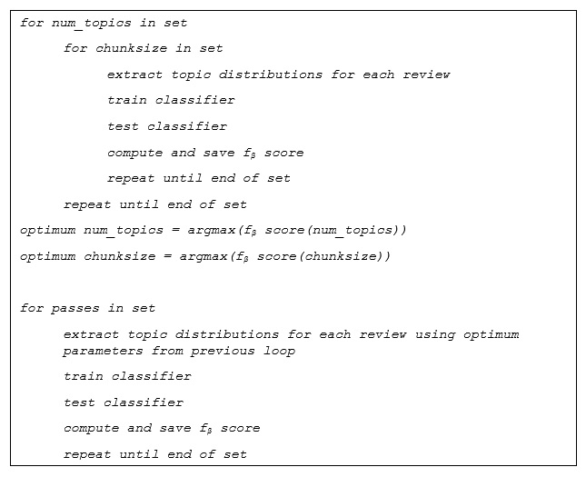
Searching through the parameter took place in two phases for both classifiers (random forests vs SVMs). The first phase looped through the number of topics and chunk size: [25, 50, 75, 100, 125, 150, 175, 200, 225, 250, 500, 1000] and [160, 320, 400, 800] respectively. I then chose the combination which yielded the best f-beta score (for each classifier) and then I ran it through a second loop for number of passes (from 1 to 15 inclusive). I broke this process in two loops to minimise execution time (one full loop takes about 25 minutes). For this stage, classifiers were set at their default values (taken from scikit-learn 0.18 suite): C = 1 with a linear kernel for SVMs and 128 estimators with maximum depth of 16 for random forests. Classifier parameters were optimised at the final stage. The whole process is summarised in the following pseudocode.
Finally, after picking the optimum parameter set for the topic model I ran the finalised topic distributions for each document through the identical grid search described for the benchmark model. The resulting maximal performance yielded the classifier with optimised parameters plus the topic model resulting in the best classification.
Results
Benchmark model
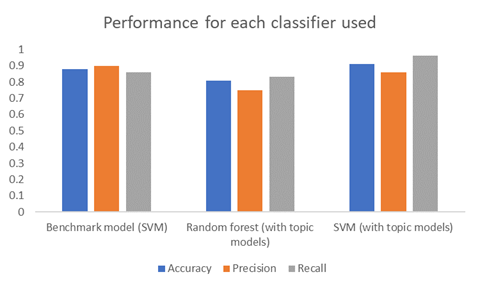
As expected the benchmark model performed quite well reaching similar levels to the Ott et al study. The best performing SVM parameters were found to be a linear kernel with a C parameter set to 10. Accuracy was reported at 0.88, precision 0.9 and recall 0.86. There were the scores to beat with the topic model methodology.
Linear kernels are estimated with weighted features. The weight values indicate the usefulness of a particular feature in discriminating between categories. For this project the features would be the tf-idf values for each bigram and the weights would indicate how much they each contribute to the discriminative power of the classifier.
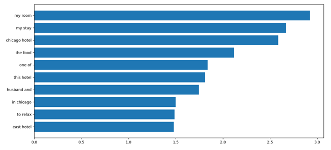
It is interesting to note that, as with the word analysis, the most highly weighted features are bigrams which are location-centric such as “in chicago” and “chicago hotel”. However the most useful features contained possessive pronouns such as “my room” and “my stay”. This might be indicative of situations where reviewers with a deceptive intent tend to avoid wording which personally links them to the object they’re trying to describe. It has also been mentioned in Ott et al that people tend to avoid using spatial descriptions in deceptive reviews.
Topic models
Out of the two classifiers tested, SVMs were the best performing ones. The SVM also outperformed the benchmark model in both accuracy (0.91) and recall (0.96).
The table below describes the best performing parameters for both random forests and SVMs after having run the optimisation procedure described in the Methods section.
| SVM | Random forests | |||
| Kernel used | RBF | Number of estimators | 500 | |
| C parameter | 0.6 | Maximum depth | 64 | |
| γ parameter | 1.0 | |||
| Number of topics | 400 | Number of topics | 400 | |
| Chunksize | 150 | Chunksize | 125 | |
| Number of passes | 10 | Number of passes | 1 |
It’s interesting to note that for both models the optimal number of topics was 400 with a similar chunksize (150 vs 125 respectively). However, there was a distinct difference in the number of passes.
Model robustness
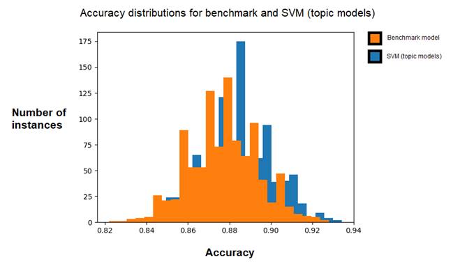
In order to ensure that the robustness and generalisation capacity of the model was within acceptable levels, I decided to further train and test it against different permutations of the dataset. Specifically, I ran the SVMTM model through a 1000 different 80-20 splits of the data and collected accuracy scores for each one. The mean accuracy was found to be 0.89 with a standard deviation of 0.017. Assuming a normal distribution, the original accuracy of 0.91 would convert to a z-score of 1.66 standard deviations above the mean. At a confidence interval of 95% we can accept that the originally reported accuracy was not significantly deviated from the sample mean and cannot be considered an outlier. This is an important piece of information because it tells us that the high performance reported initially was not specific to the particularities of the original dataset split but within the wider accuracy distribution of the permutation samples.
Further comparisons with the benchmark model revealed an average accuracy of 0.87 with a similar standard deviation score of 0.016. Using a Kolmogorov-Smirnoff two-sample test, which is safe under non-normal assumptions, I found that SVMTM accuracy scores were consistently and significantly higher (D = 0.18, p << 0.01) than the benchmark model’s.
Conclusions
The purpose of this project was to find a classifier capable of detecting and discriminating between truthful and deceptive hotel reviews. Looking at the single word analysis there were no differences in either the word distribution or word type between the two categories. This meant that whatever method I used it would have to rely on higher-level properties of the documents. To this end, I decided to use topic models as a means to extract useful latent features from the text. These latent features would in turn provide a solid basis for classification.
On the surface, topic modelling seems to have had the desirable effect. I was able to classify truthful from deceptive reviews successfully with a 91% accuracy (which is greater than the 88% value set by the benchmark classifier). However, if we look into the predictive value of the different approaches then comparisons become less clear-cut.
To put this in quantitative terms, I first took the precision of the benchmark and SVMTM classifiers. Precision is the conditional probability of the condition being true (i.e. truthful review) given a positive prediction. We can convert this to something more tangible by computing the information entropy of the precision value (which is probabilistic in nature) and then subtracting from the unconditional entropy of the categories (assuming both categories are equally probable which might not be necessarily true).

What tells us is the amount of information we gain given a classifier’s prediction or in other words, the reduction in uncertainty regarding whether a review is truthful or not. The information ceiling is 0.69 (which is the total unconditional entropy of the categories ).
Following on this, I calculated an information gain of 0.36 bits for the benchmark model and 0.29 bits for SVMTM. This means that the benchmark is actually more informative when it makes a positive prediction compared to SVMTM. The opposite was true when I repeated the same procedure for the negative predictive value. I found 0.3 bits and 0.56 bits for the benchmark and SVMTM respectively. Taking the average of these values for each respective classifier I found an average of 0.33 for the benchmark and 0.425 for SVMTM. Collectively, this means that predictions made by SVMTM are more informative compared to the benchmark model.
It would also be useful to be able to assign a monetary value on the classifier’s performance. For example, one question we could ask is: how much money does the user save for each correct prediction made? Is there a difference in value between true positive and true negatives?
Unfortunately, there is no additional data which can provide specific monetary losses for each misclassified review. We can, however, emulate different cases using synthetic data. Let us suppose the hotel management reports a $10 gain for each true positive review and a $5 gain for each true negative. Furthermore, it reports a $50 loss for each false positive and $20 loss for each false negative. This could be the case where allowing a falsely legit review would damage the reputation of the hotel more so than rejecting a genuine one (in the latter case there would be no spam ultimately posted online). We can then multiply each monetary value with the corresponding metric and sum across all products. The table below summarises all the metrics.
| Actual + | Actual – | Actual + | Actual – | |
| Predicted POS | 0.96 × $10 | 0.04 × -$50 | 0.86 × $10 | 0.14 × -$50 |
| Predicted NEG | 0.12 × -$20 | 0.88 × $5 | 0.1 × -$20 | 0.9 × $5 |
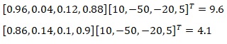
Summing across all products I found that with SVMTM a user would report savings of $9.6 per decision made and $4.1 with the benchmark model. Comparatively, a user would report a loss of -$27.5 in the case of a dumb classifier picking the correct class only 50% of the time.
This example only serves to illustrate that the choice of classifier largely depends on the relative costs per decision. As the results stand in the present case, one could pre-emptively pick the SVMTM classifier since it performs more accurately and is more informative but at the same time bear in mind that different cases might necessitate different approaches.
Addendum
This is a follow-up to the work been done so far and it specifically touches on how we can further improve the classifier’s performance by applying a form of feature selection. To do this, I computed the mutual information for each bigram in the corpus and then removed bigrams which did not pass a certain threshold. The information threshold was set at 0.055 (13% of features removed).
A distribution of accuracies to see where we stand.
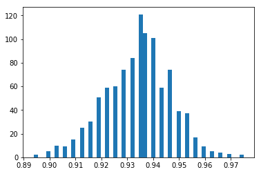
Not bad.
First of all, this outperforms the 88% average accuracy of the benchmark model.
Secondly, this procedure basically highlights the importance of feature selection. The procedure which comes out of this is: 1) tokenize the review, 2) remove the bigrams we’ve found which contain little to no information, and then 3) extract topic distribution for the review (and simultaneously updating the topic model itself). Finally, we can classify the processed document using the optimised classifier parameters.
References
Blei, D., & Lafferty, J. (2007). A correlated topic model of Science. Annals of Applied Statistics, 17–35.
Blei, D., & Lafferty, J. (2009). Topic Models.
Jindal, N., & Liu, B. (2008). Opinion spam and analysis. Proceedings of the international conference on Web search and web data mining, (pp. 219-230).
Ott, M., Cardie, C., & Hancock, J. (2013). Negative Deceptive Opinion Spam. . Proceedings of the 2013 Conference of the North American Chapter of the Association for Computational Linguistics: Human Language Technologies.
Ott, M., Choi, Y., Cardie, C., & Hancock, J. (2011). Finding Deceptive Opinion Spam by Any Stretch of the Imagination. . Proceedings of the 49th Annual Meeting of the Association for Computational Linguistics: Human Language Technologies.
Steyvers, M., & Griffiths, T. (2007). Probabilistic Topic Models. In T. Landauer, D. McNamara, & S. Dennis, Handbook of Latent Semantic Analysis . Psychology Press.
