Language: MATLAB 8.3
Packages: Statistics and Machine Learning Toolbox, SPM8
Methods: fMRI processing & analysis, general linear modelling, supervised learning, DISTATIS, k-means clustering

---

The brain is an extremely complex, biological system. It is comprised of about 100 billion neurons over an area of 2000 cm² (that’s about 15 million neurons per square centimetre). The sum-total of connections between neurons vastly outnumbers the tally of stars in the Milky Way. But of course the story doesn’t end there. These biological units, known as neurons, are themselves computational nodes capable of basic operations. Combined together in ensembles, their intricate dynamics give rise to phase oscillations and other large-scale phenomena.

And yet within this apparent mess of neurons, glial cells and action potentials an entire, unique world appears as rich and complex as the actual world we inhabit. Any attempt to get a grasp on the mechanics which give rise to our mental lives must be meticulous and methodical, much like any other science. But where studying the chemical composition of a pulsar 5 million light years away from our planets has its own charm, when it comes to studying the brain things are more personal, more intimate. Traversing these vast, unexplored vistas is no easy feat. It’s no surprise then that to tackle the task on hand, the overarching question of “how does the brain work?” is fractionated into hundreds of simpler yet more focused sub-questions: “how does language work?”, “how does memory work?”, “how does vision work?”. And the fractionation goes even further, in an almost fractal-like fashion, addressing individual facets of each cognitive function, each with their own nuances, their own world of expertise: “what is the primary function of the inferior temporal cortex?”, “how does symbol-grounding taking place (if it does at all..)?” and so and so forth, almost ad infinitum…

All this done so that one day all the answers from all these questions will coalesce seamlessly into one grand theory of the brain. That’s what one hopes at least…

One can wax philosophical and ponder these question from the comforts of his armchair, fireplace crackling by his side, a glass of sherry in hand. But to answer it we need data. Lots of data. And this is where the intersection between data science and neuroscience comes in. You pose a question, acquire data, analyse it and then assess whether you have a plausible explanatory hypothesis on your hands (which hopefully makes its way to a publication).

So what sort of data are we dealing with here? Traditionally, the cognitive sciences relied upon behavioural experiments whereby the participant engaged in a task, (for example naming a presented picture) and then collecting reaction times and error rates. That’s all great but now with the advent of neuroimaging technologies we have the choice of directly peering into the inner workings of the brain. There are various non-invasive brain imaging methods such as EEG (electric encephalography) and MEG (magnetic encephalography). The particular method I was using is known as functional magnetic resonance imaging or fMRI for short.

I am really boiling the technicalities to a very basic level here, but the following is a gist of how it works. As a matter of fact, fMRI is actually a prime example of how advances in a different field of science have inadvertently lead to breakthroughs in another field. In this case, advancements in medical physics allowed neuroscience researchers to take advantage of the magnetic inhomogeneities of deoxygenated and oxygenated blood and use it as a basis for imaging the brain in vivo. The general working mechanism behind fMRI is that as blood rushes into active brain areas there is an increase in oxygenated blood. This is turn leads to a decrease in deoxyhaemoglobin which has paramagnetic properties (meaning it distorts the magnetic signal of the surrounding brain tissue). This imbalance between oxy- and deoxy-haemoglobin, technically known as the blood-oxygenation-level-dependent or BOLD signal, is what the fMRI apparatus is picking up.

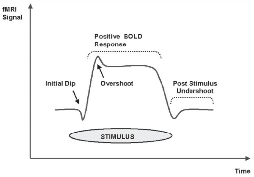
BOLD signal shows initial dip and then a more prolonged ‘positive’ signal (adapted from Kesavadas and Thomas, 2008)

It’s important to note that the signal itself is not neuronal activity but rather symptomatic of it. An encouraging set of results by Logothetis et al had shown that this assumption need not rely on pure faith: the authors presented a strong correlation between direct electrophysiological activity and fMRI. So we can safely assume that the BOLD signal is a good proxy for neuronal activity although the exact nature of its source remains a hot topic in the neuroimaging field.

The particular question I addressed over my PhD can be put quite simply as “how do we extract meaning from things we see in the world?”. In other words, how do we make sense of this barrage of seemingly chaotic and noisy data we receive through our senses? Where do we encode this information we extract from our visual environments? And furthermore, is it possible to decode this information from recorded brain activity?

The challenge now is to take this BOLD signal described earlier and determine via an array of analytical tools whether it contains information regarding a particular task. In my case, the task at hand was naming a sequence of images shown in the scanner. The purpose was to see whether we could decode high-level information regarding these particular images directly from the recorded brain activity. With this mind I will address each of the stages involved in the project life cycle in the following sections.

Theoretical background

The first step was to extract a set of feature-based concept-specific properties. Concepts in this context are assumed to be points within a multi-dimensional geometrical space (Shepard, 1974). By doing so geometrical properties in the space (e.g. length of the vector, the angle between two vectors) can signify important featural measures of concepts such as sharedness or correlational strength.

Exploring the geometrically-derived conceptual space in this manner allowed me to extract a novel measure which in this study I termed as cLength. Much like other, more familiar measures, cLength captures specific feature-based aspects of a concept’s structure. Most importantly, cLength captures both sharedness and correlational strength which means that it provides a more comprehensive description of a concept’s semantic structure. The general focus of this project was to try and demonstrate a rigorous relationship between the categorical organization of conceptual representations, neural responses and cLength. This was done in order to establish whether the measure had any relevance to our understanding of how the brain organizes conceptual information and also whether it could account for this organization better than previously used measures. Furthermore, such a relationship would also warrant future usage of the measure in subsequent studies.

Sample feature vectors for five randomly drawn concepts. Blue color denotes 0 (or the absence of a feature in the concept) and red denotes 1 (or the presence of a feature).

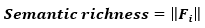
A point in this f-dimensional vector space represents a particular object. The length (or Eucliean norm) of a feature vector, F_i, in this case is directly proportional to the number of features or the semantic richness (Taylor et al., 2012) of a concept:

Geometric properties derived from this vector space are restricted to the features characterising each concept. Mapping the concepts onto the cross-product vector space incorporates the relationships between a concept and all other concepts in the space within a particular vector. To derive the cross-product vector space I multiplied the concept matrix, M, with its transpose, M^T:

Schematic depicting the matrix multiplication of the feature matrix and its transpose resulting in cross-product matrix.

The above operation resulted in C = MM^T which is a 517 × 517 square matrix such that each element in its row vector C_i indicates the number of common features between some concept n and another concept m. For example, elements for the ‘dog’ concept vector would be ‘bat’ = 3, ‘goat’ = 6, ‘octopus’ = 1 and ‘trolley’ = 0.

This vector representation allows for a more rich description of objects which takes into account not only the number of features but also how the concept relates to all other concepts in the space. The length of a concept vector C_i within the space was derived as:

This measure encapsulates not only the semantic richness (i.e. the number of features) but also the mean distinctiveness (i.e. how shared on average are the constituent features of the concept) as well as the number of concepts that it shares at least one feature with. It is thus a particularly information-rich measure.

Next, I correlated semantic similarity and feature statistics. The aim was to understand whether feature statistics had any effect on the arrangement of concepts in the semantic space, as determined by the overlap of feature content. I first extracted the distance matrix for the whole set of concepts (517 × 517) using 1 – cosine distance as the metric (the semantic distance measure used by McRae et al (2005) and others). Multidimensional scaling (MDS) is a way to construct a ‘map’ showing the relationships between different objects on a low-dimensional plane given a matrix of distances (or dissimilarities) between them – in this case a distance matrix where each element denotes the cosine distance between any given pair of concepts. The inter-point distances on the map approximate the original distances as described through the distance matrix. The dimensions of the map itself reflect a projection which maximally preserves distances in the original distance matrix – what matters are the relevant distances between points rather than absolute distances (e.g. is A closer to B than A is to C?). For the purposes of this study I used classical MDS which takes as its input a distance matrix and returns a set of orthogonal vectors which describe different aspects of the data. For the purposes of the study I extracted two principal axes for visualising the semantic space. I then correlated each of the two dimensions with the feature statistics described above.

Below is a plot of the first two principal dimensions of the semantic similarity matrix (1 – cosine) which result from the classical MDS algorithm. Animals and tools are color coded in red and green respectively. The size of the points denotes the cLength value corresponding to the concept. Bar plot in figure b shows the Pearson’s correlation values between conceptual structure variables and the two dimensions resulting from classical MDS. **/* denote significance at p < 0.01 and p < 0.05 respectively.

The arrangement of concepts within the semantic similarity space is significantly related with cLength. This means that concepts sharing a significant degree of features (giving rise to categories) also possess similar cLength values.

Purpose

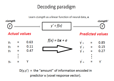
For this project I wanted to relate cLength and neural activity that goes in the brain when we recognise a visual object. Specifically, I want to know where this information might be encoded and how reliable is our decoding algorithm.

To this end, I used a linear decoder trained on fMRI data and used it to predict a given object’s properties.

Data acquisition

The first stage was to gather enough participants to put through the MRI scanner. Typically for these studies, 15-20 volunteers is a good number to work with. During selection I had to ensure that participants were suitable for fMRI (e.g. no dentures, pacemakers, metal prosthetics etc.), had no language issues (e.g. dyslexia) and were fit to take part (e.g. no serious diseases such as meningitis, not pregnant etc.).

During the experimental session, the participant had to look at a sequence of images depicting everyday objects and name them in succession. The corresponding brain activity (i.e. BOLD signal) was recorded as a continuous signal throughout the whole duration of the experiment. As a result of this procedure, I ended up with 15 BOLD signal datasets, one for each participant.

Data preparation / Data wrangling

In neuroimaging lingo, this step is collectively called pre–processing. There are several things we need to take care of before we even begin applying any learning algorithms. During a typical fMRI session, an image is taken of the entire brain about every 2 seconds. Given that a participant might move his/her head (even slightly!)  over this period of time we need to make sure that all these brain images taken from a single participant are aligned together. This step is called spatial re-alignment and it is absolutely crucial before any further processing takes place.

Next, we need to appreciate that every brain is different. How can we be sure that one point-coordinate in one’s head is the same in another’s? We need to have a universal point of reference where each participant’s imaged brain is aligned unto the same coordinate system. The coordinate system, or atlas, used in this study is known as the MNI (after Montreal Neurological Institute) system and has been in use since the early 2000s. After we’ve taken care of this step, known as normalisation, we can then move on our analysis.

Alright, so now we have a bunch of raw imaging data which has been re-aligned and normalised. It’s generally good to clean it up a little bit so now it’s a good time to apply high-pass filtering to remove physiological effects such as respiratory noise, heartbeat etc.

The data is now ready for some preliminary statistical analysis. First we need to know how well does the BOLD signal correlate with a given image (or condition in experimental parlance). The basic assumption here is that the brain won’t respond to all stimuli in the same way. There will be a variability in response from stimulus to stimulus. What we need at this point is a measure of how well does the signal relate to the stimulus. The general linear model (GLM) is an equation which expresses the observed response variable (i.e. BOLD signal) in terms of a linear combination of explanatory variables:

Y = βX + ε

This allows us to relate what we observe to what we expect to see. We can solve this equation either by some optimisation method or numerically using the following equation:

β’ = (X^TX)^-1X^Ty

Now that we have the analytical tools in place we need to run this GLM for each stimulus and for each participant. The β-estimates we get as a result of this (one per stimulus per participant) form the data used in any further analysis.

Finally, there is the issue of the signal-to-noise ratio. Like any other large dataset worth its salt, fMRI data are riddled with noise, the source of which can range from pulmonary / cardiovascular distortions to discrepancies in tissue-to-air ratios. One way to increase our signal is by averaging across all our participants’ β-estimates and hope that the process will reduce variations within individual participants. Another, more typical way, is known as smoothing and it’s usually performed at early stages before we apply the GLM. For this process, a Gaussian kernel is applied to each point (or voxel) in the brain map. It efficiently accounts for anatomical variability but it assumes that no information is lost in this locally averaged component, i.e. all information is contained within a low spatial-frequency band. For the intents and purposes of this study, we don’t want to make this assumption and so that’s why in this case we skipped smoothing.

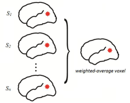
Individual participant β-estimates for each stimulus were averaged across participants using DISTASTIS (Abdi, 2001). This averaging methodology assigned weights to each participant’s data based on how close they were to the overall mean. All subsequent analyses were carried out on this final, weighted-averaged image. In the image below, a voxel is merely the 3-dimensional equivalent of a pixel because we are effectively dealing with a stereotaxic representation of the brain.

Now that we have our data, processed and ready for analysis, we can move on to the next stage.

Hypothesis & Modelling

A linear decoder was trained on the weighted-averaged  β-estimates to decode visual object properties (i.e. cLength within the context of the experiment) with leave-one-out cross-validation.

To make sure that any found relationship between response and property was not “polluted” by other covariates there was an additional step of residualisation. In other words, I removed all linear dependencies between voxel responses and other properties which were unrelated out property of interest. Voxel responses were residualised with respect to the phonological length of the object name, visual complexity of the stimulus, category membership and naming accuracy.

The correlation, D(y,y’), between actual and predicted values was then used as a metric of information content. Significance values were obtained by permutation testing (n = 1000) whereby the order of values within predictor x (the voxel response) was randomised at each permutation. The norm of the residuals was then collected for each permutation to give rise to a null distribution.

Evaluation

After we’re done performing the decoder algorithm on all voxels in our brain map we’re left with two key questions – how strong are the effects and where are they localised?

To assess performance significance we need to set an appropriate p-value threshold. In addition, we also need to bear in mind that given the high number of comparisons, one for each voxel in the brain, there will be a considerable number of false positives. For this reason, we apply a corrective method known as FDR (false detection rate) which adjusts our threshold value accordingly.

The correlation map depicts only cLength-sensitive voxels at p < 0.05 (FDR-corrected for multiple comparisons).

So what exactly is going on here? First of all most of the effects are localised within a region known as the inferior temporal cortex, localised in the lower right for the left-side image and lower left for the right-side image. This is a centre involved with high-level processing of visual objects. So at least we know that the location of the effects makes sense in light of already existing knowledge. There’re also effects in a region called the primary motor cortex, near the top the brain, which is a region involved in representing motor commands and other related properties.

Secondly, if we wished we would be able to extract reliable information regarding visual objects by applying our simple decoder described earlier. We wouldn’t need to know what object the participant is observing – we would be able to decode this just by looking at his/her brain image data!

That’s great but the neuroscientist in me has a couple of other questions. As you might’ve noticed in the image above, there are two spatially distinct clusters – one near the bottom of the brain (lateral in brain imaging terminology) and other near the top (or dorsal). Now, the question is, do these regions possess different pattern of response? Although there is significant information encoded in these regions this does not necessarily imply that they encode it in the same way.

To answer this question, I performed an additional unsupervised clustering analysis on these effects to reveal any distinct clusters of voxel responses.

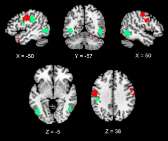
K-means clustering revealed two distinct clusters of response within the set of informative voxels voxels. Cluster 1 (green) is mostly centred within the lateral, inferior temporal cortex (bottom of the brain). Cluster 2 (red) is mostly centred the dorsal clusters (top of the brain). A minor sub-cluster (part of Cluster 1) was also detected within dorsal clusters.

What this tells us is that it appears that the clusters are not separated spatially but also in the way they encode information about visual objects.

Overall comments

So, what did we learn from all this? Well, first from a strictly pragmatic viewpoint we now know it’s perfectly possible to effectively decode information from just looking at the activity of human brains (using fMRI of course). But in addition to that, if we’re interested in the hows and whys of brain function, we’ve also learned that some informaiton at least is encoded linearly within certain regions. Furthermore, the k-means clustering analysis revealed that the activation profile of these voxels is largely dependent on their location (lateral vs dorsal clusters).

References

Abdi, H., O’Toole, A. J., Valentin, D., & Edelman, B. (2005). DISTATIS: The analysis of multiple distance matrices . Computer Vision and Pattern Recognition Workshops (pp. 42-42). IEEE.

Ashby, F. G. (2011). Statistical analysis of fMRI data. MIT press.

Marouchos, A. (2016). The nature of conceptual representations in the visual object processing system, University of Cambridge

McRae, K., Cree, G. S., Seidenberg, M. S., & McNorgan, C. (2005). Semantic feature production norms for a large set of living and nonliving things. Behavior research methods , 37 (4), 547-559.